
Styling and symbology
Before we begin
Section titled “Before we begin”Before diving into this module’s exercises, it would be good if you can review and familiarize yourself with styling layers and making maps. You can also look at advanced styling and symbology techniques.
Multi-variable symbologies
Section titled “Multi-variable symbologies”1.1. Bivariate choropleth map of barangays showing population density and annual population rate
Section titled “1.1. Bivariate choropleth map of barangays showing population density and annual population rate”
What we want to achieve
Section titled “What we want to achieve”- A map of Quezon City barangays showing both the population growth rate (2000 to 2020) and the people per 100 square meters.
What we have
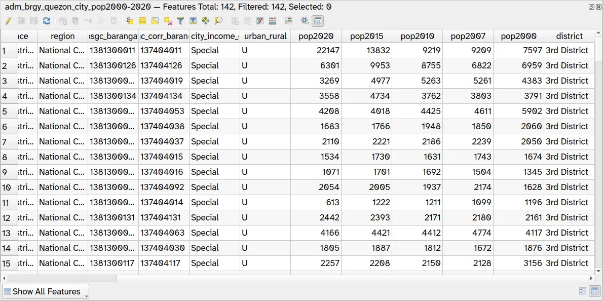
Section titled “What we have”- adm_brgy_quezon_city_pop2000_2020 - the barangay-level admin boundary data generated from a previous exercise with population from 2000 to 2020
Relevant QGIS knowledge/skills
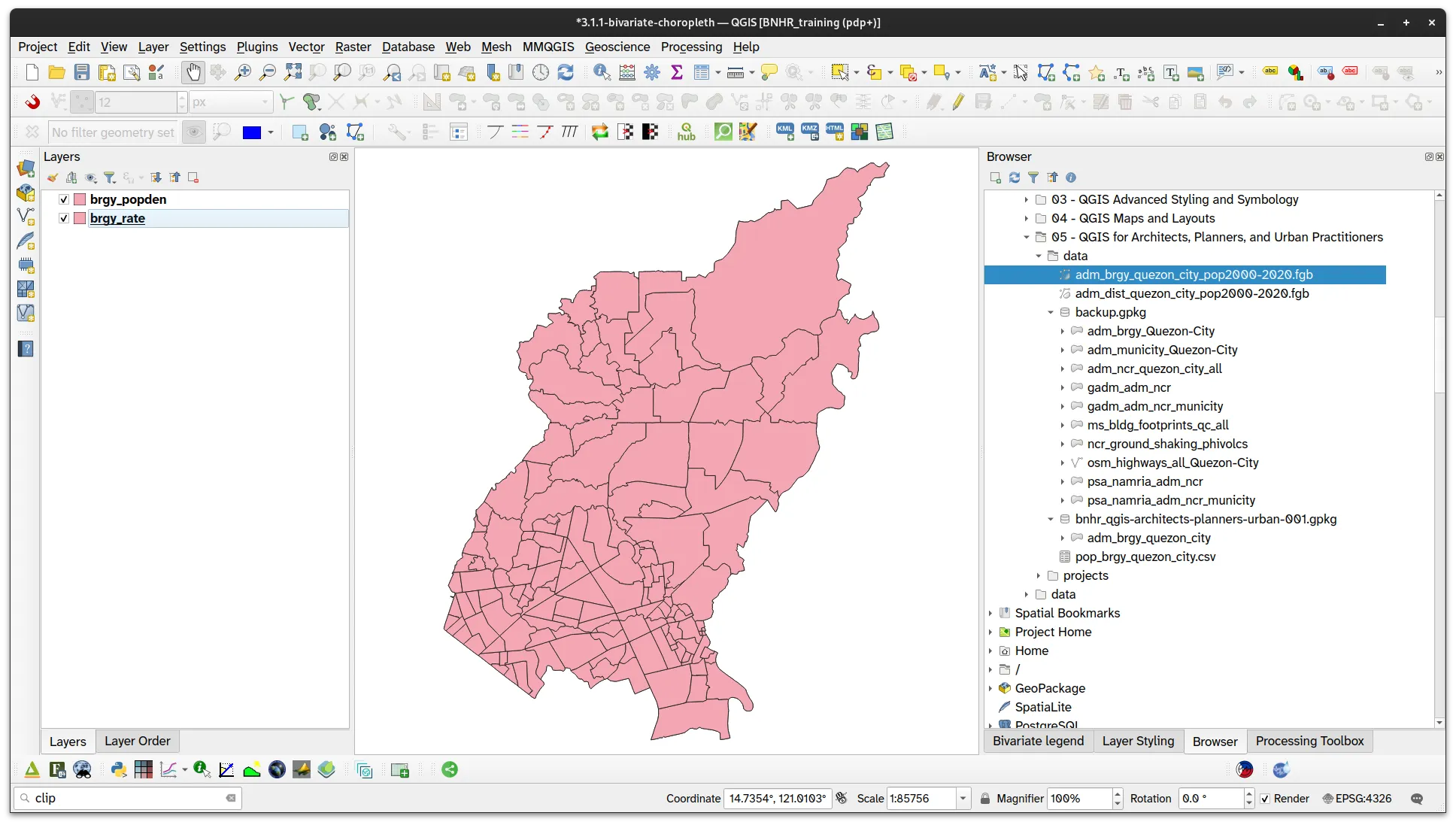
Section titled “Relevant QGIS knowledge/skills”- Load the adm_brgy_quezon_city_pop2000_2020 layer. Make sure that it already has the fields for population from 2000 to 2020.
- Duplicate the adm_brgy_quezon_city_pop2000_2020 layer. Since we’ll be creating a bivariate choropleth map using blending modes, we need 2 vector layers to show. In this case, we’ll show the annual population growth from 2000-2020 and the number of people per 100sqm in the barangay. Name the two layers brgy_rate and brgy_popden.
-
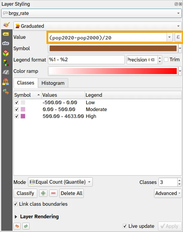
Next, we make a choropleth map for the brgy_rate layer using a Graduated symbology using the following parameters.
- Symbology: Graduated
- Value:
(pop2020-pop2000)/20
- Classes
- Low
- Color: #e8e8e8
- Values: -500.00 - 0.00
- Moderate
- Color: #dfb0d6
- Values: 0.00 - 500.00
- High
- Color: #be64ac
- Values: 500.00 – 5000.00
- Low
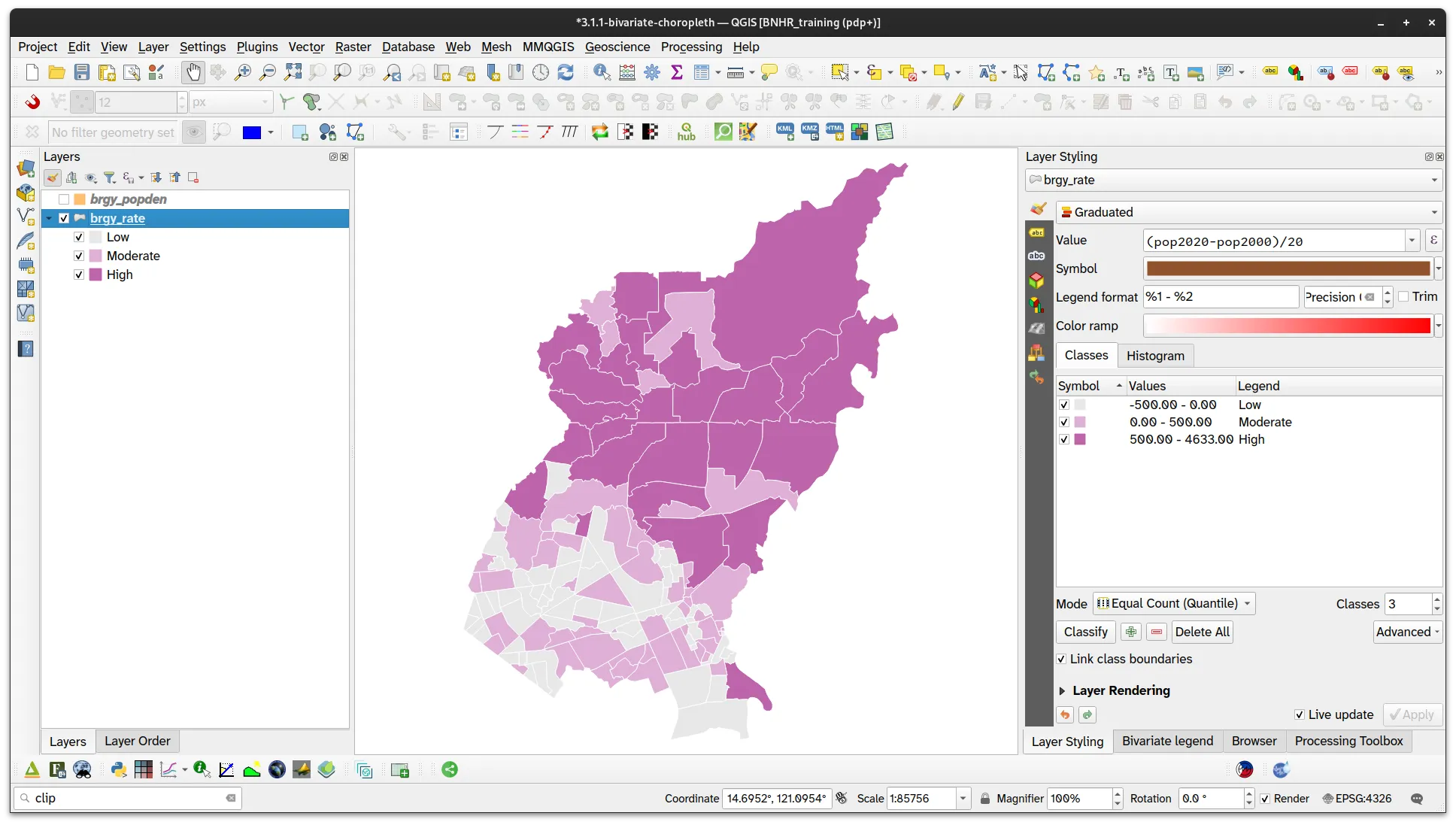
- Your brgy_rate layer should look like:
- Do the same for the brgy_popden layer but our parameters will be:
- Symbology: Graduated
- Value:
100*pop2020/$area
- Classes
- Low
- Color: #e8e8e8
- Values: 0.000 - 1.500
- Moderate
- Color: #ace4e4
- Values: 1.500 - 3.000
- High
- Color: #5ac8c8
- Values: 3.000 - 15.000
- Low
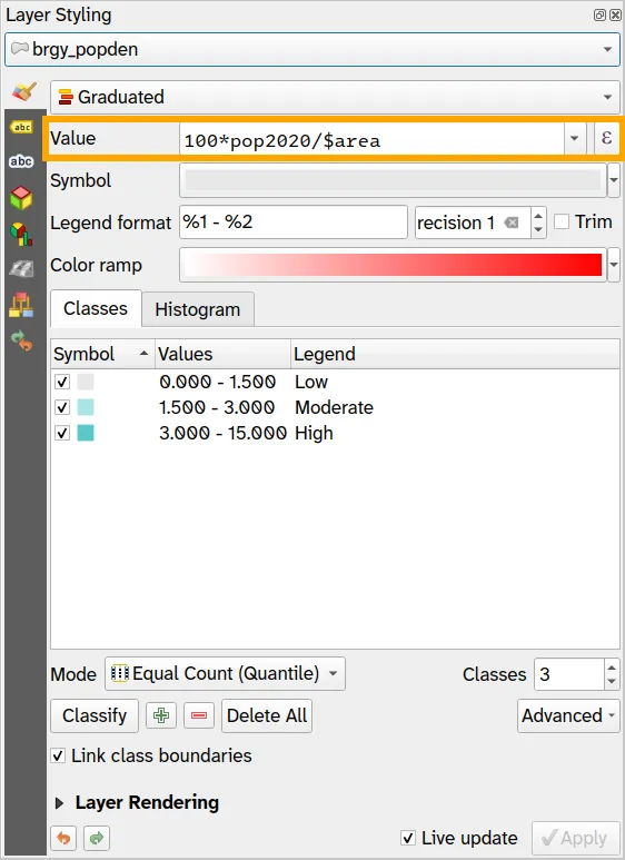
- Your brgy_popden layer should look like:

- Now that you have the two choropleth maps, create the bivariate choropleth effect by changing the blending mode of the top layer (brgy_popden) to Multiply.


1.2. Using both size and color to communicate information about the districts
Section titled “1.2. Using both size and color to communicate information about the districts”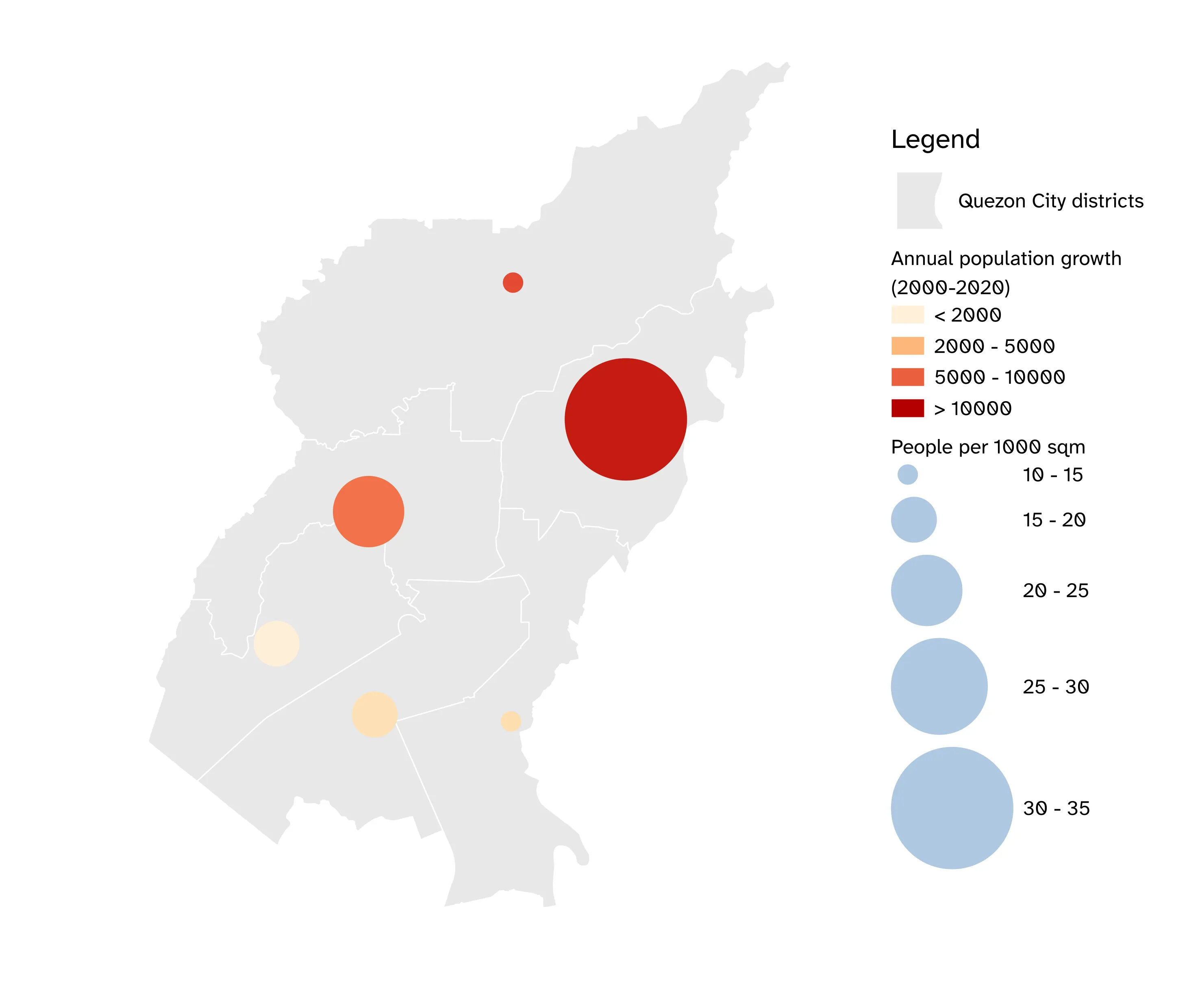
What we want to achieve
Section titled “What we want to achieve”- Use circles to show population information about districts in Quezon City where the size pertains to the people per 1000 sqm and the color indicates the annual population growth from 2000 to 2020.
What we have
Section titled “What we have”- adm_dist_quezon_city_pop2000_2020 - the district-level admin boundary data generated from a previous exercise with population from 2000 to 2020
Relevant QGIS knowledge/skills
Section titled “Relevant QGIS knowledge/skills”Option 1 - Geometry generator approach
Section titled “Option 1 - Geometry generator approach”- Load the adm_dist_quezon_city_pop2000_2020 and duplicate the layer.
- Rename one base and apply a simple single symbol symbology.
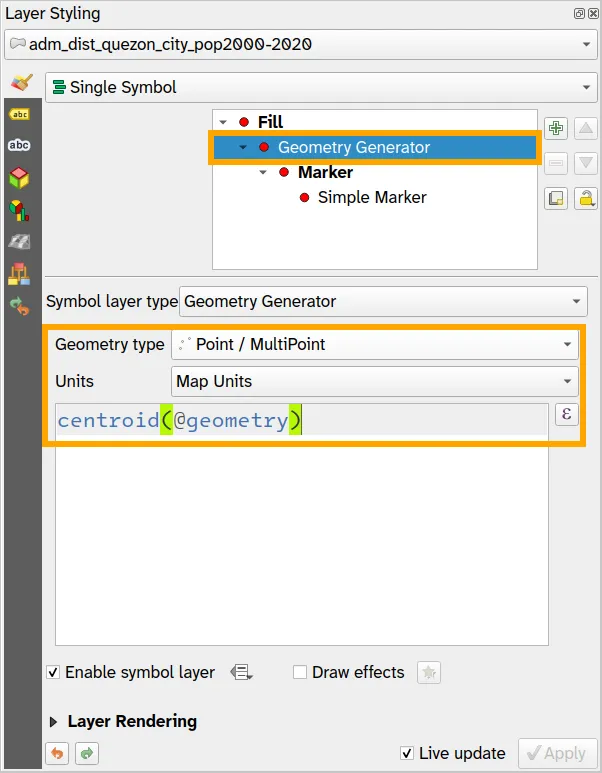
- On the other layer, selece Geometry Generator as its Symbol layer type.
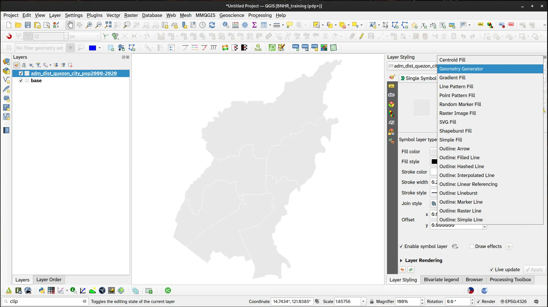
- Change the Geometry type to Point/MultiPoint and use the following expression to generate a centroid:
centroid(@geometry)
- On the Simple Marker, use the Assistant to override the Size parameter.
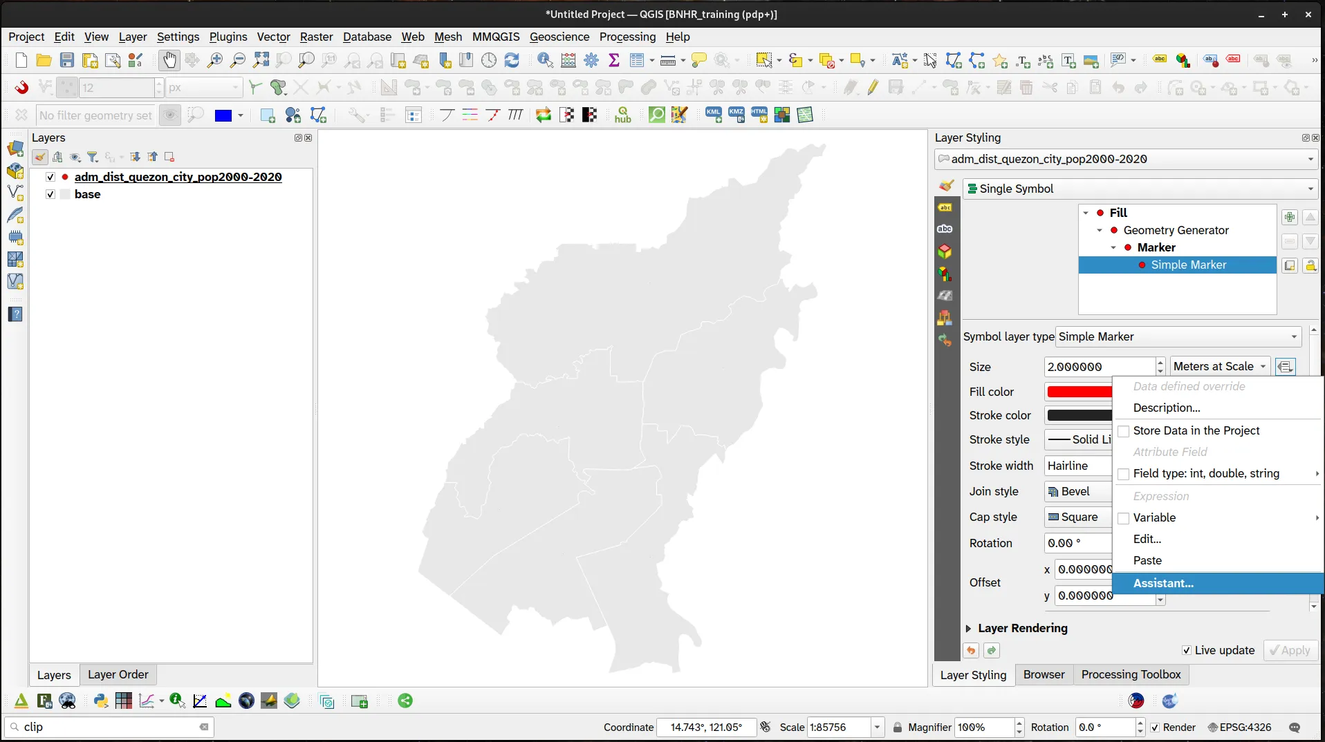
- Use the following parameters:
- Source
1000*pop2020/$area
- Values from 10 to 35
- Output
- Size from 500
- to 3500
- Source
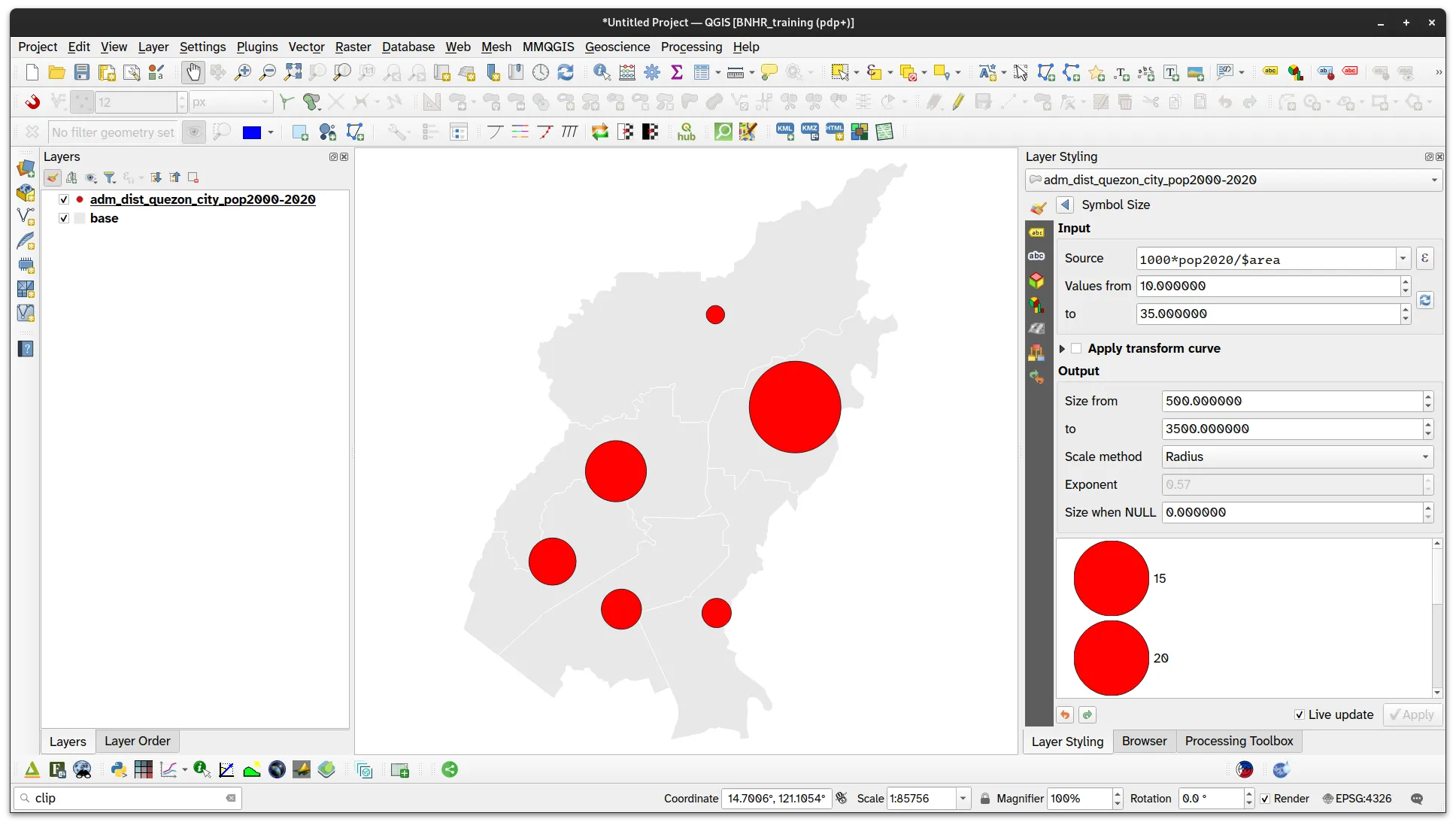
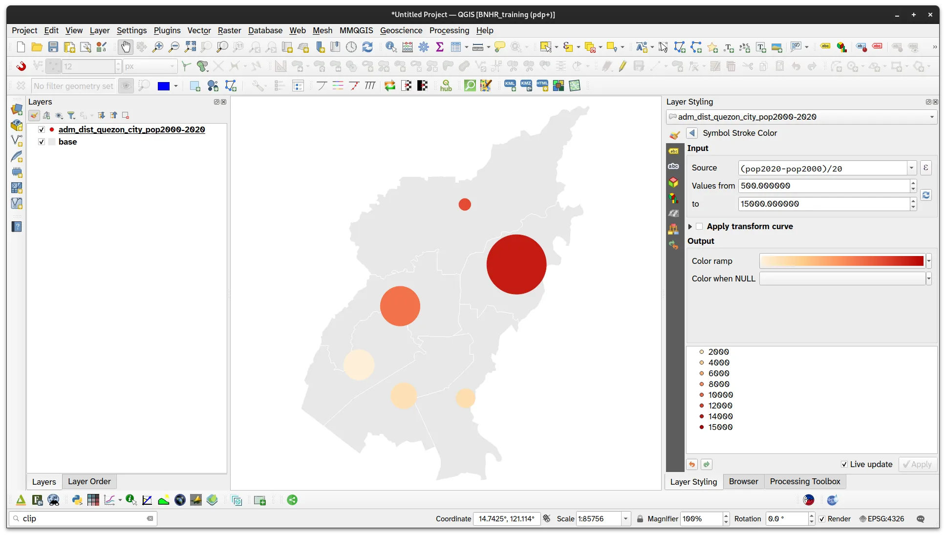
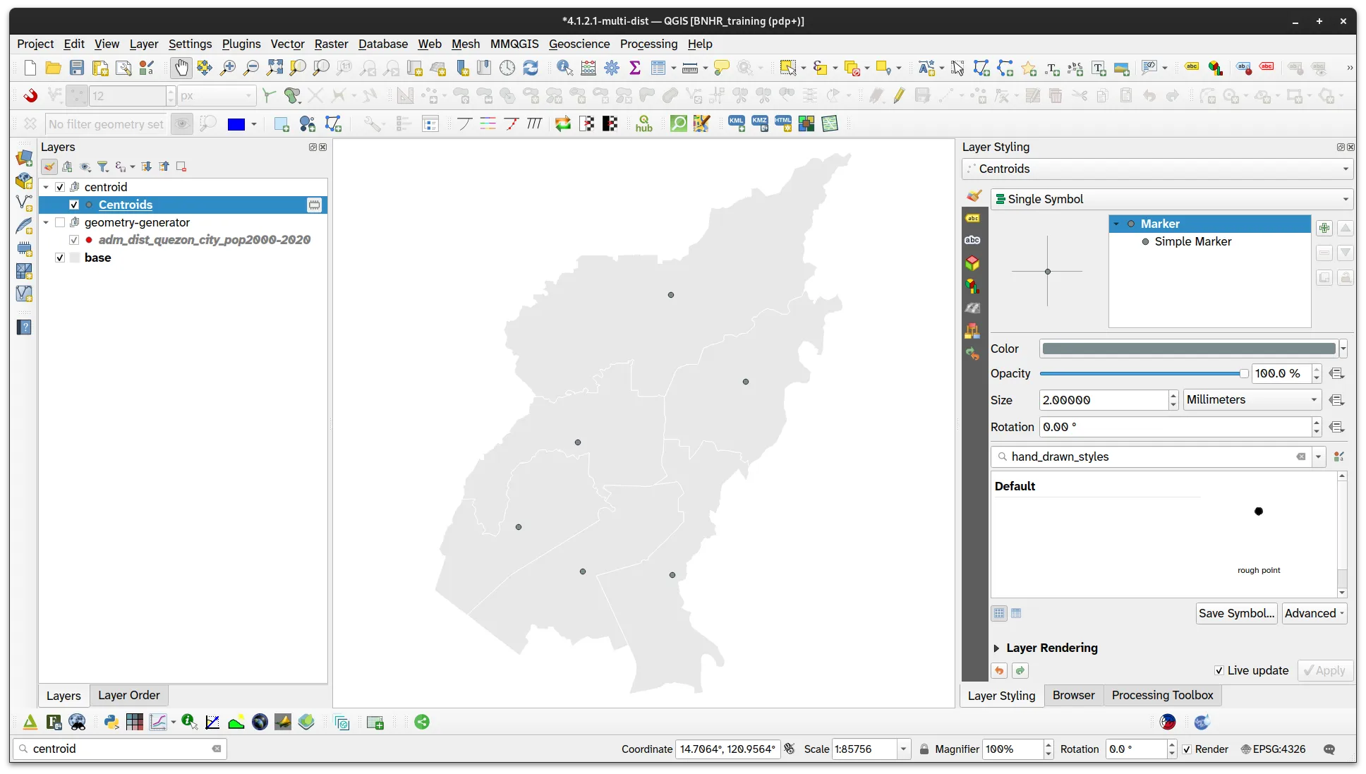
- Your layer should now look like below:
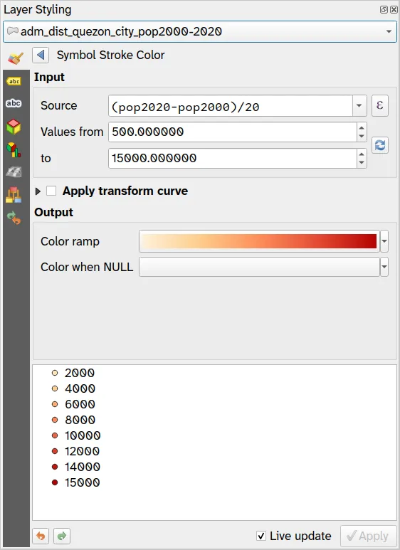
- Next, let’s use the Assistant to override the Symbol Fill and Symbol Stroke Color parameters.

Option 2 - Centroid approach
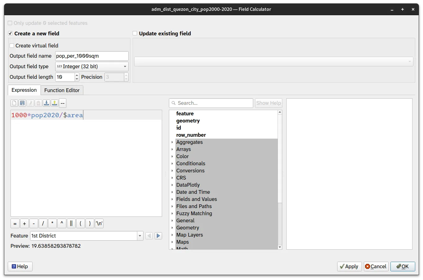
Section titled “Option 2 - Centroid approach”- Add a new field to the adm_dist_quezon_city_pop2000_2020 layer to hold the number of people per 1000 square meters using the following expression:
1000*pop2020/$area
- Run the Centroid processing algorithm to create a new point layer (centroid) based on adm_dist_quezon_city_pop2000_2020.
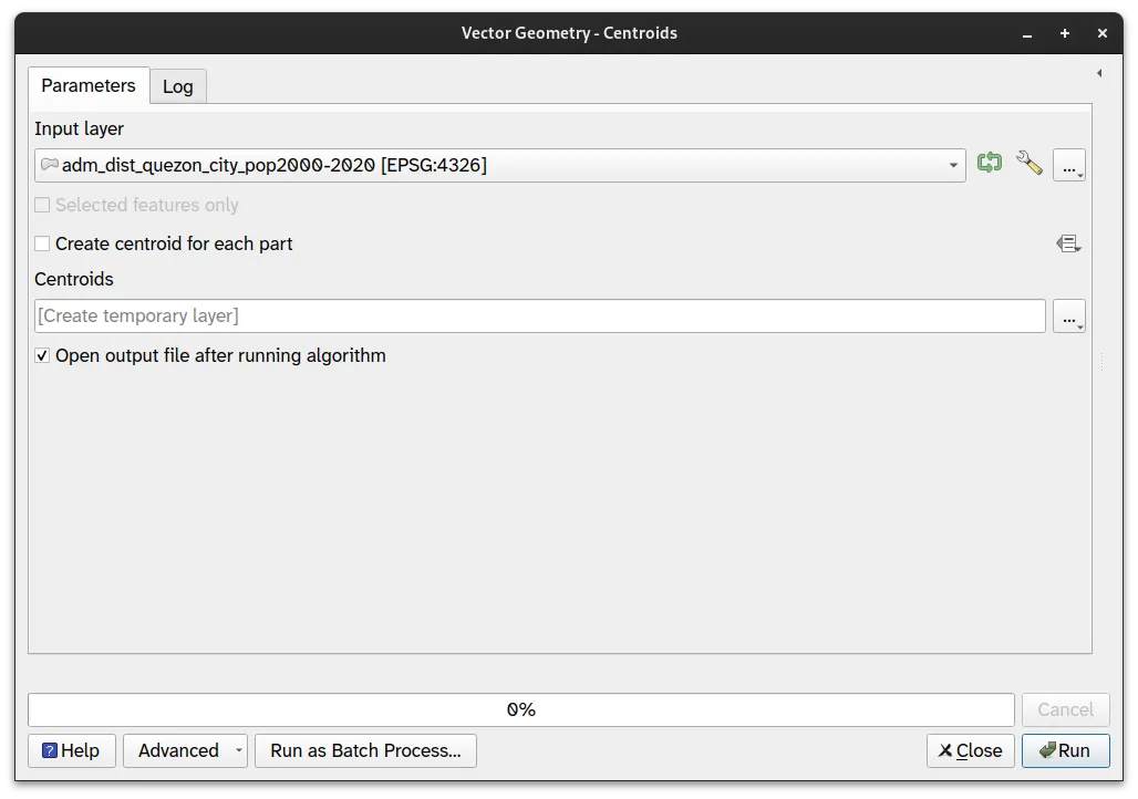
- A new layer (Centroid) should be created.
- Apply a Graduated symbology and use the following parametres:
- Value: pop_per_1000sqm
- Method: Size
- Size from: 500 to 3500 Map Units
- Classes:
- 10 - 15
- 15 - 20
- 20 - 25
- 25 - 30
- 30 - 35
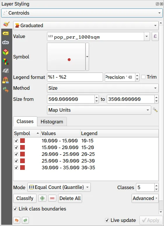
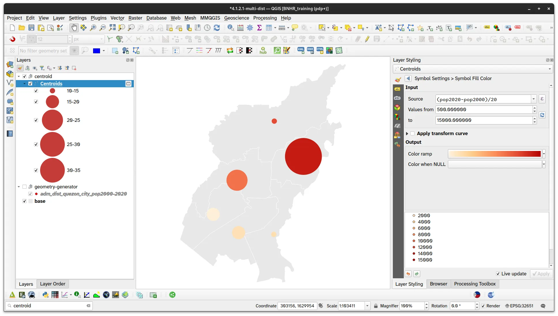
- Your Centroid layer should look like below:

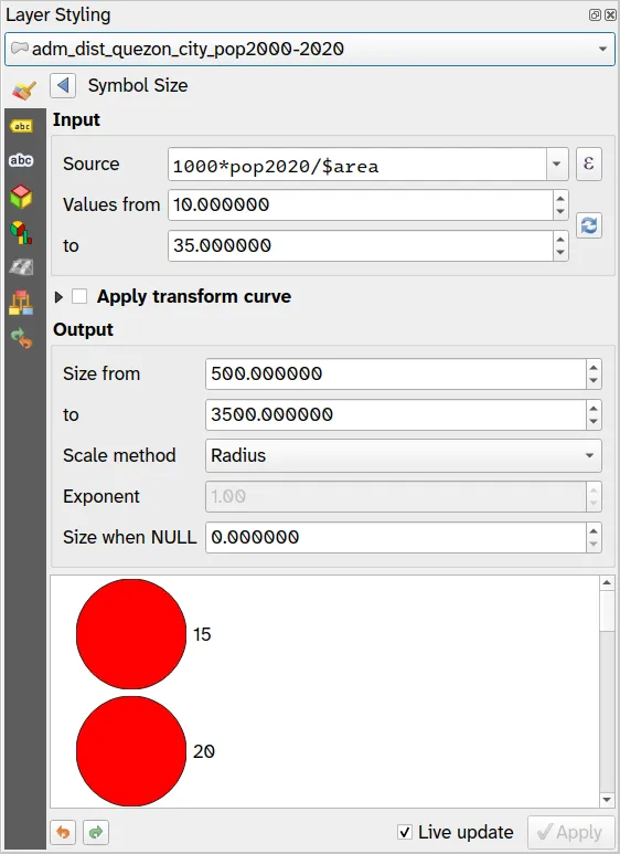
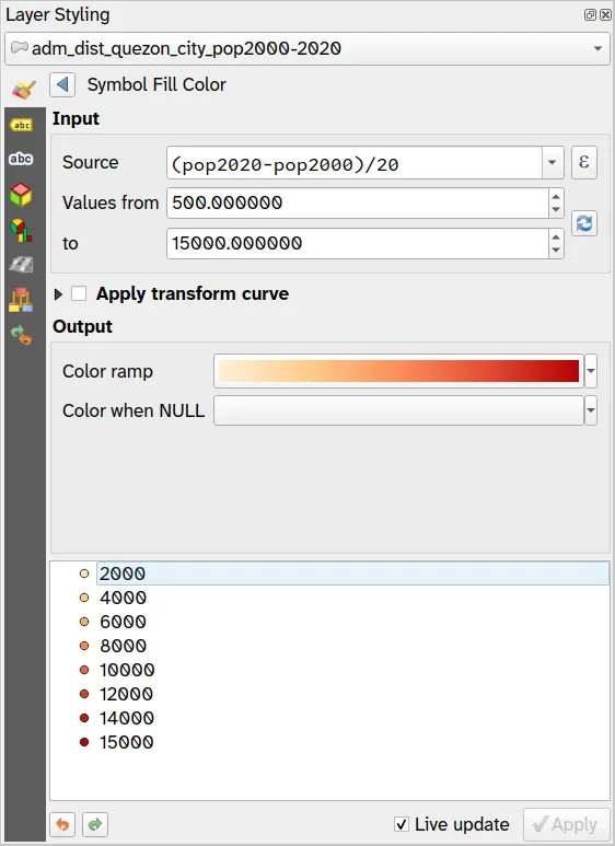
- Use the Assistant to override the Symbol Fill Color with the following parameters:
- Source:
(pop2020-pop2000)/20
- Values from: 500 to 15000
- Source:
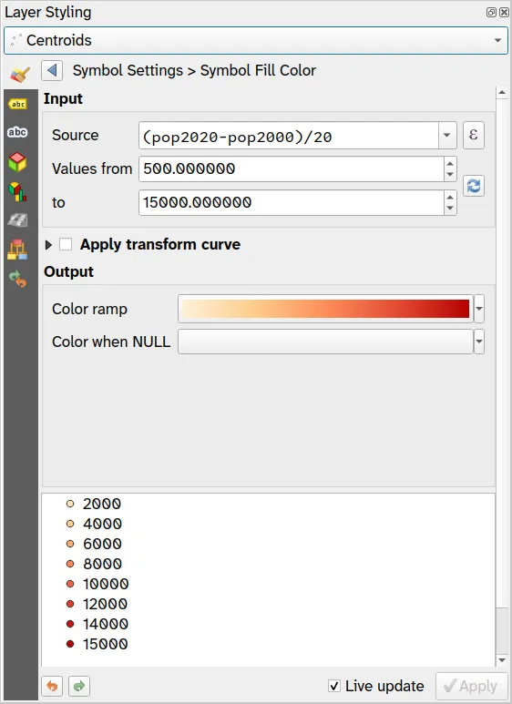
- Your layer should look like below:
Rule-based and scale-dependent symbologies
Section titled “Rule-based and scale-dependent symbologies”2.1. Styling roads and land-use using rules and symbol levels
Section titled “2.1. Styling roads and land-use using rules and symbol levels”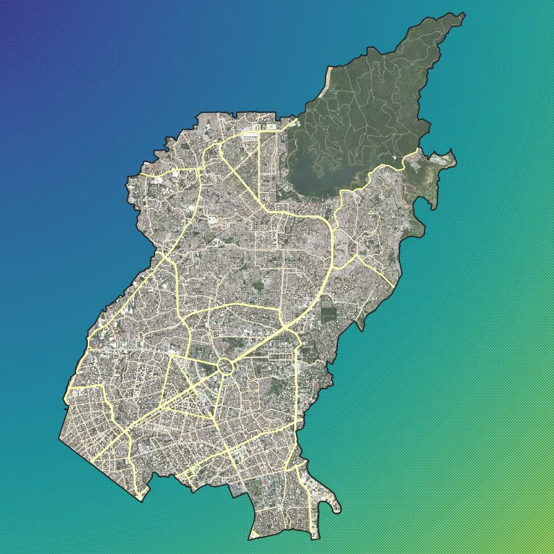
What we want to achieve
Section titled “What we want to achieve”- Style a road network similar in style to the ones we see in web maps by applying rule-based symbology on OpenStreetMap road data.
- Apply the same symbology to multiple landuse categories.
What we have
Section titled “What we have”- adm_municity_quezon_city
- osm_roads_quezon_city
- osm_landuse_quezon_city
- Other relevant layers:
- satellite image basemap
Relevant QGIS knowledge/skills
Section titled “Relevant QGIS knowledge/skills”- Load the adm_municity_quezon_city, osm_roads_quezon_city, and osm_landuse_quezon_city layers.
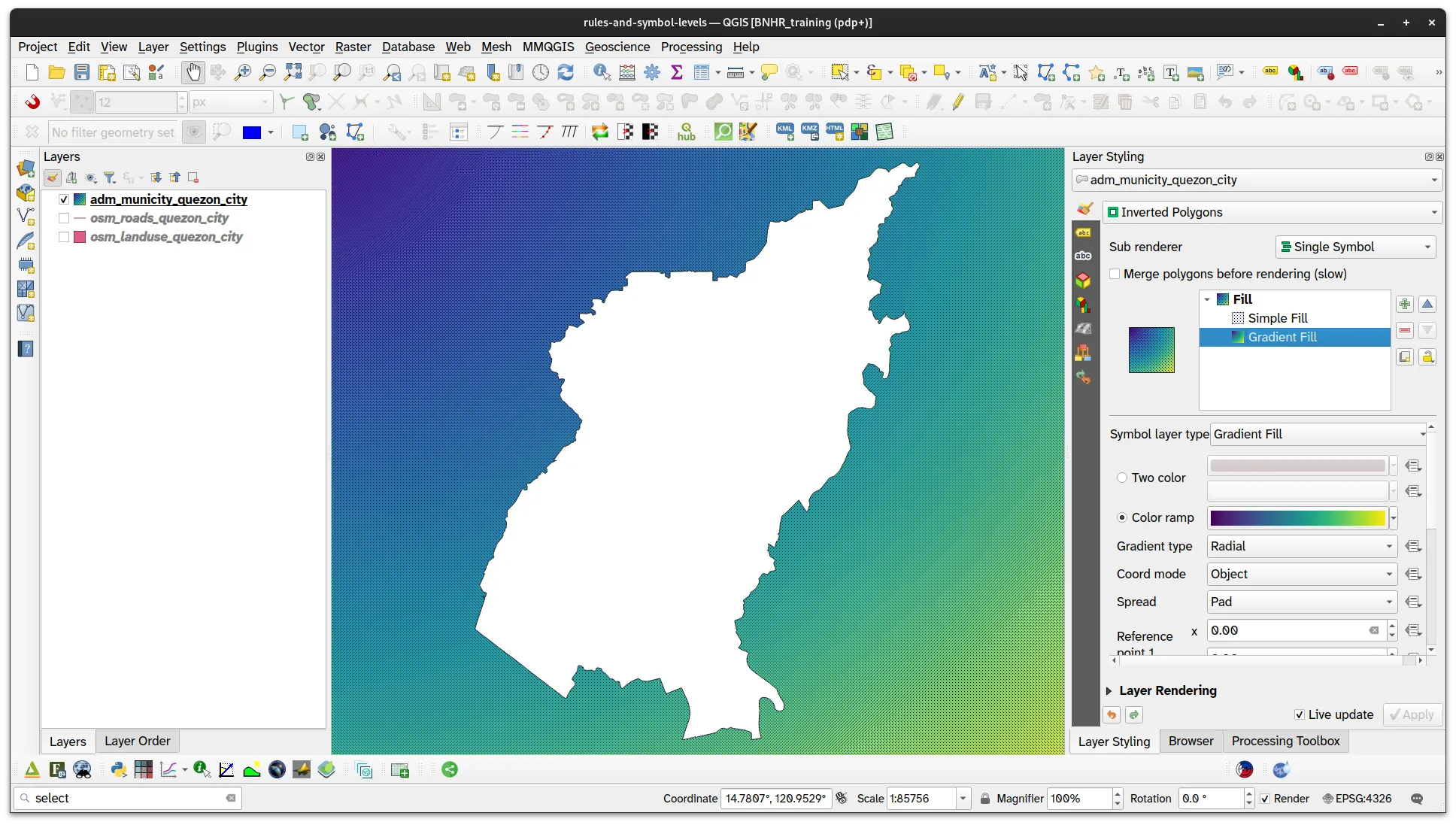
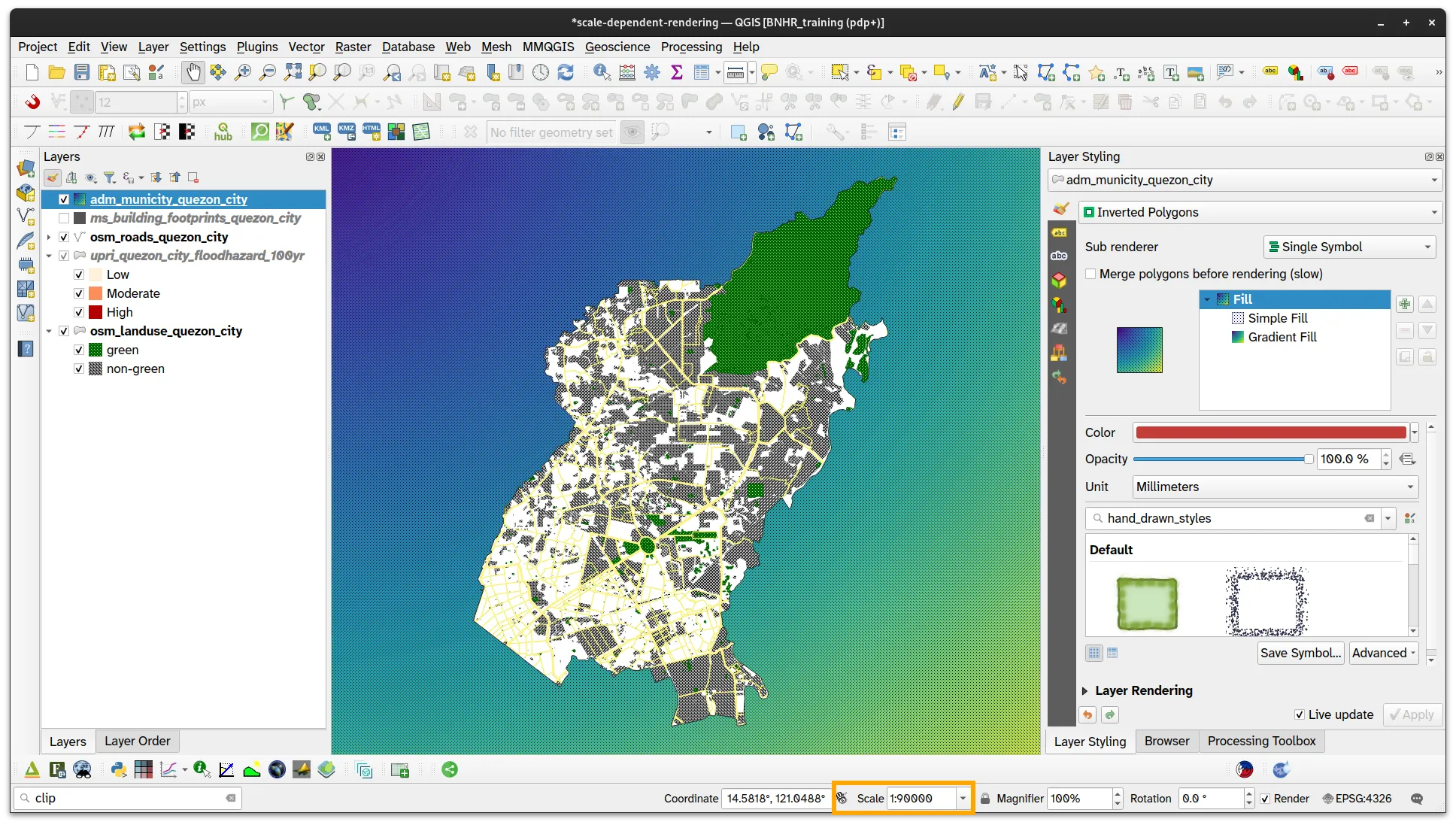
- Style adm_municity_quezon_city using Inverted Polygons and apply two fills (a Simple Fill and a Gradient Fill).
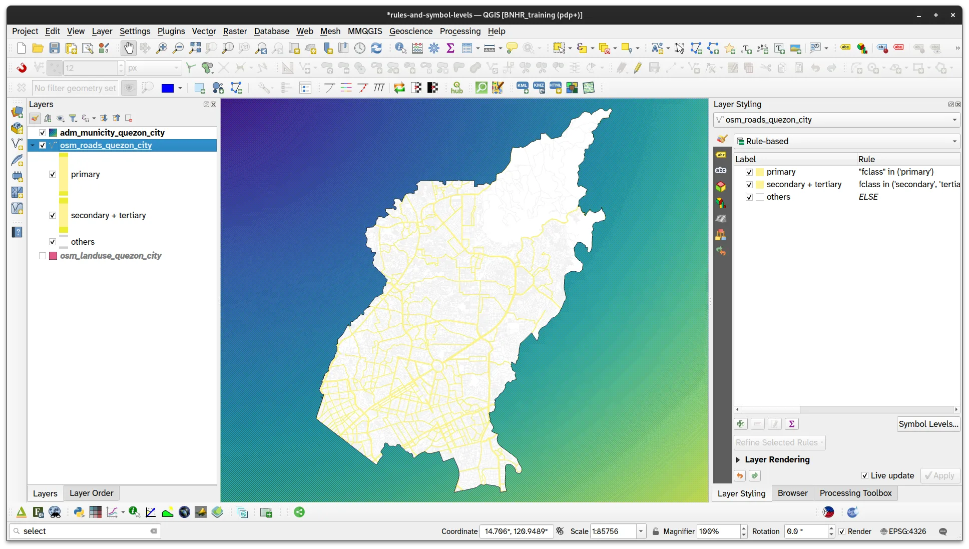
Apply rule-based symbology to the road network data
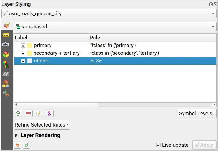
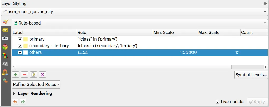
Section titled “Apply rule-based symbology to the road network data”- For the osm_roads_quezon_city layer, you will create 3 rules—one for primary roads, another for secondary roads, and a catch-all (for everything else). The rules will be:
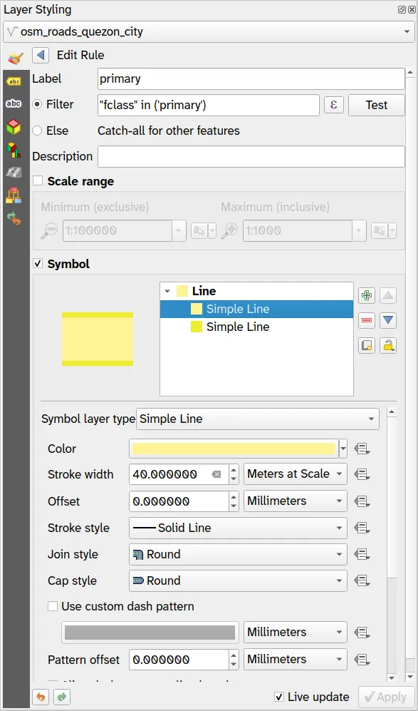
- Primary roads:
- Label: primary
- Filter:
"fclass" in ('primary')
- Symbol:
-
Simple Line (1)
- Color: #fff495
- Stroke width: 40 meters at scale
- Stroke style, Join style, Cap style: Solid line, Round, Round
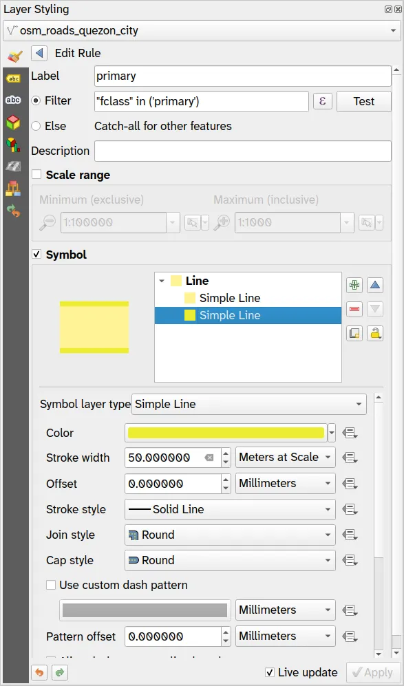
-
Simple Line (2)
- Color: #ecec32
- Stroke width: 50 meters at scale
- Stroke style, Join style, Cap style: Solid line, Round, Round
-
- Primary roads:
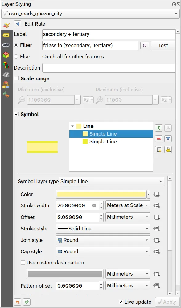
- Secondary and tertiary roads:
- Label: secondary and tertiary
- Filter:
fclass in ('secondary', 'tertiary')
- Symbol:
-
Simple Line (1)
- Color: #fff495
- Stroke width: 20 meters at scale
- Stroke style, Join style, Cap style: Solid line, Round, Round
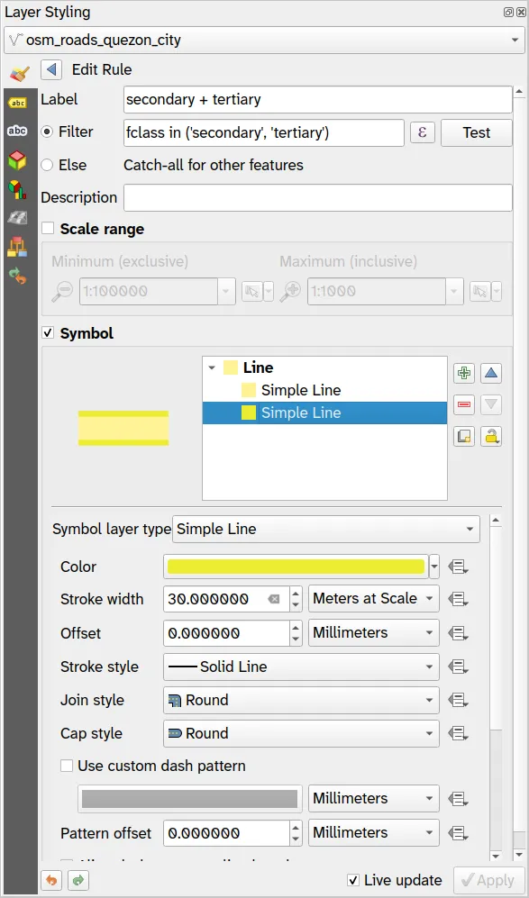
-
Simple Line (2)
- Color: #ecec32
- Stroke width: 30 meters at scale
- Stroke style, Join style, Cap style: Solid line, Round, Round
-
- Other roads:
- Label: others
- Filter:
Else
- Symbol:
- Simple Line (1)
- Color: #ffffff
- Stroke width: 8 meters at scale
- Stroke style, Join style, Cap style: Solid line, Round, Round
- Simple Line (2)
- Color: #d3d3d3
- Stroke width: 12 meters at scale
- Stroke style, Join style, Cap style: Solid line, Round, Round
- Simple Line (1)
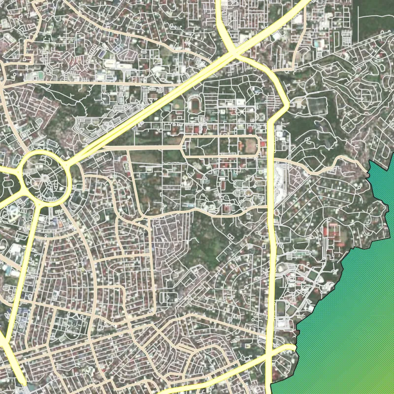
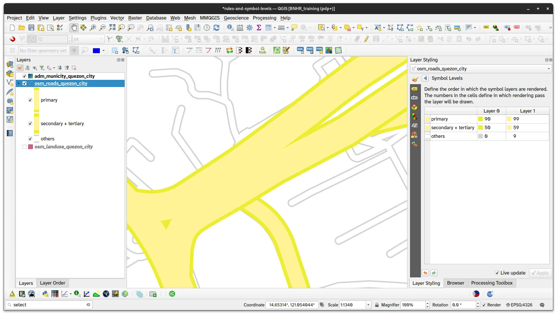
However, if you zoom in to the map, you will notice a bit of an issue.
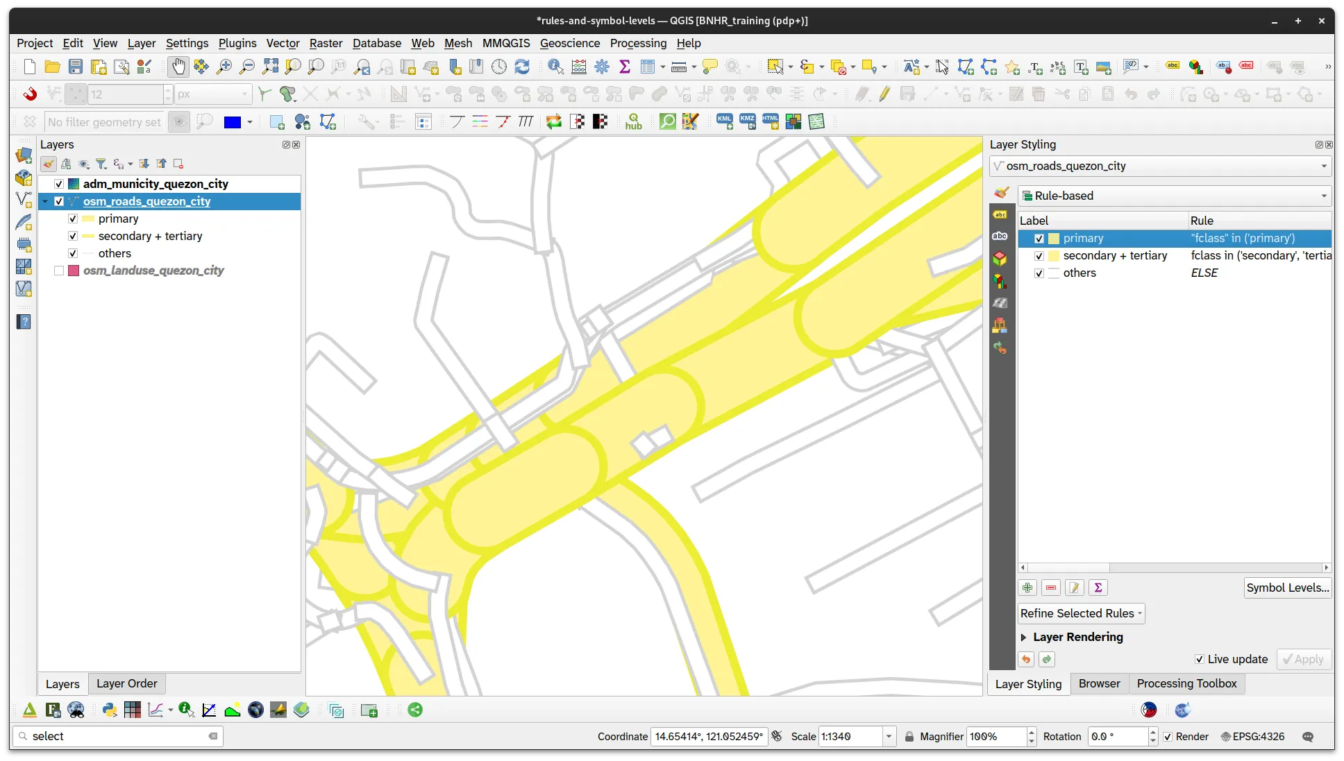
If you look real close, you will notice that the different road feature overlap in a poor way. What you want to do is control the rendering order so that the primary roads are rendered over the secondary and other roads while the secondary roads are rendered over the other roads. To do this, you can use Symbol Levels.
Rendering roads consistently and cleanly using Symbol Levels
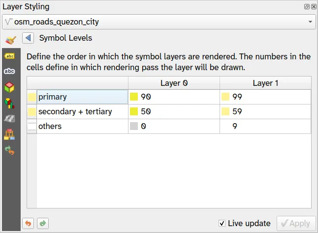
Section titled “Rendering roads consistently and cleanly using Symbol Levels”Symbol Levels allow you to define the order in which the symbols are rendered. The numbers assigned to symbol rules define when they will be rendered, that means a lower number is rendered first and a higher number will be rendered on top of it. Using this, you can ensure that the other roads are rendered at the bottom and the primary roads are rendered on top.
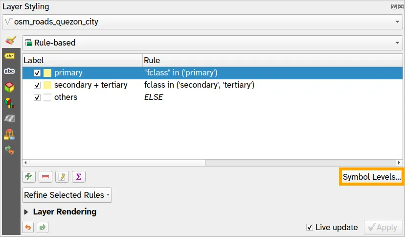
- Click Symbol Levels on the Layer Styling panel or the layer Properties of the osm_roads_quezon_city layer.
- Update the Symbol Levels for each of the rules. Make sure that the values for primary are the highest while the values for Others are the lowest.
- With these symbol level rules applied, your road layer should look like below when zoomed in.
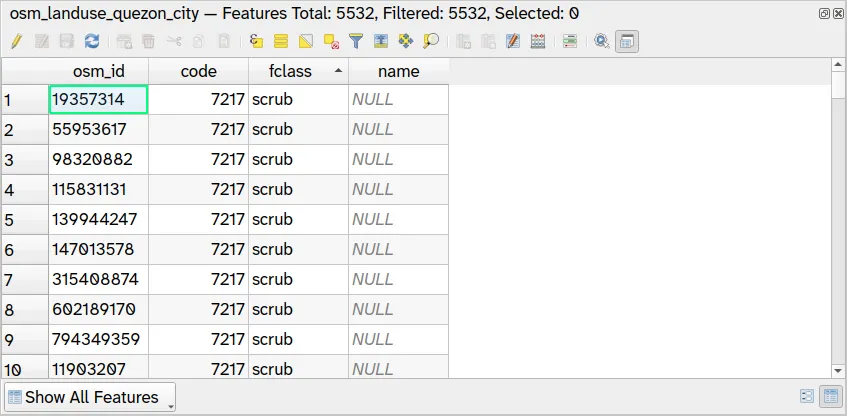
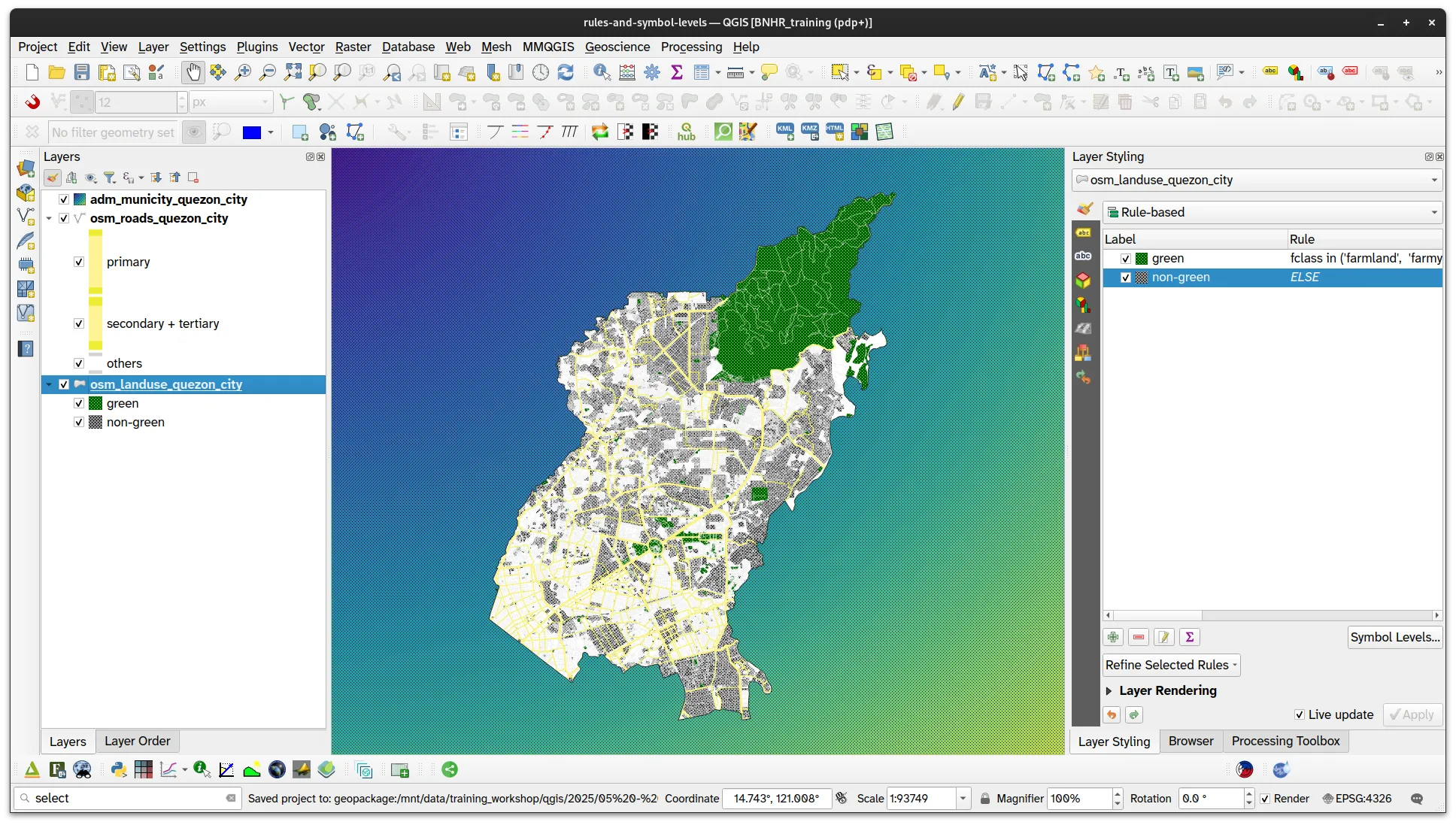
Apply rule-based symbology to the landuse data
Section titled “Apply rule-based symbology to the landuse data”Activate the osm_landuse_quezon_city and notice that there are several land use classes available.
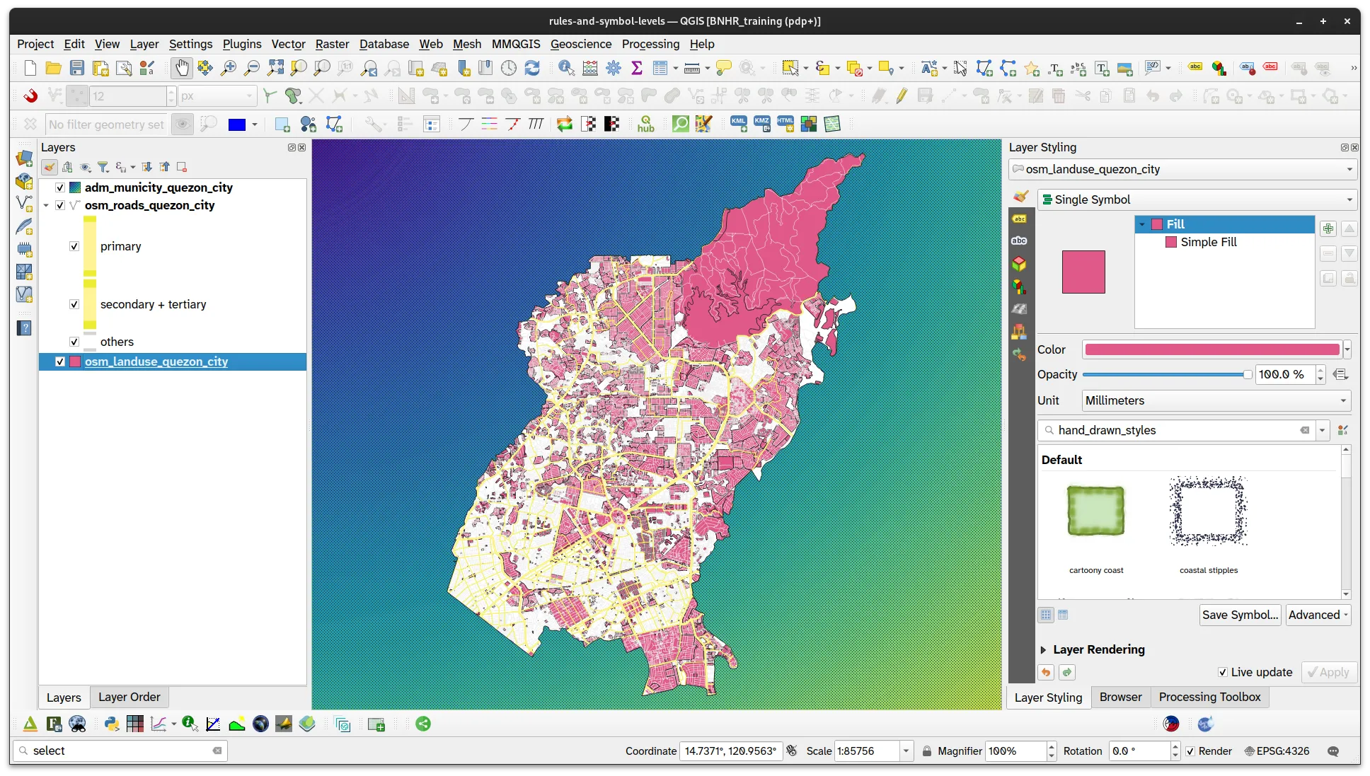
In this case, we want to style only the “green” areas. We can do this by applying a rule-based symbology.
-
Select the landuse layer.
-
Select Rule-based for the symbology type.
-
Add a new rule using the green arrow.
-
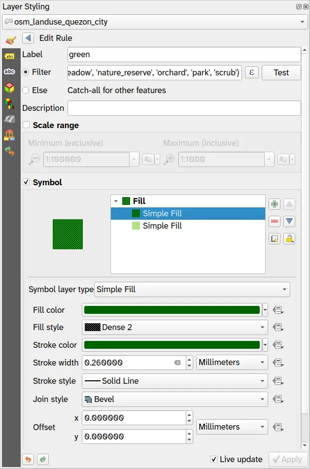
Use the following rule:
- Label: green
- Filter:
fclass in ('farmland', 'farmyard', 'forest', 'grass', 'meadow', 'nature_reserve', 'orchard', 'park', 'scrub')
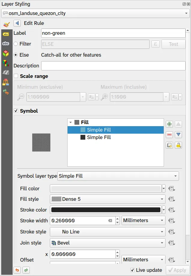
- Add another rule as a catch-all. Style this catch-all as below.
2.2. Showing different features at different zoom levels
Section titled “2.2. Showing different features at different zoom levels”What we want to achieve
Section titled “What we want to achieve”For this exercise, your goal is to change which features and layers are shown as you zoom in or out of the map. In a way, you will be changing the level of detail in the map depending on the zoom level. For example:
- When zoomed out (e.g. scale < 1:50,000): you only want to see the primary, secondary, and tertiary roads as well as the green areas.
- At middle zoom level (e.g. scale between 1:25,000 and 1:50,000): you want to add the other roads as well as the flood hazard layer.
- When zoomed in (e.g. scale > 1:25,000): you want to show all layers including the osm_buildings.
What we have
Section titled “What we have”- adm_municity_quezon_city
- osm_roads_quezon_city
- osm_landuse_quezon_city
- upri_quezon_city_floodhazard_100yr
- ms_building_footprints_quezon_city
Relevant QGIS knowledge/skills
Section titled “Relevant QGIS knowledge/skills”Scale-dependent visibility
Section titled “Scale-dependent visibility”The trick here is to use Scale Dependent Visibility. In QGIS, you can fine-tune and control the scale range at which layers and features become visible.
- For layers: you can find this in the Rendering tab of the Layer Properties
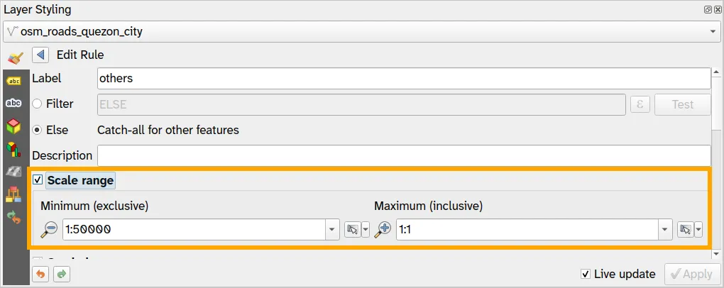
- For features styled using rule-based symbology: you can specify the minimum scale and maximum scale in the style settings.
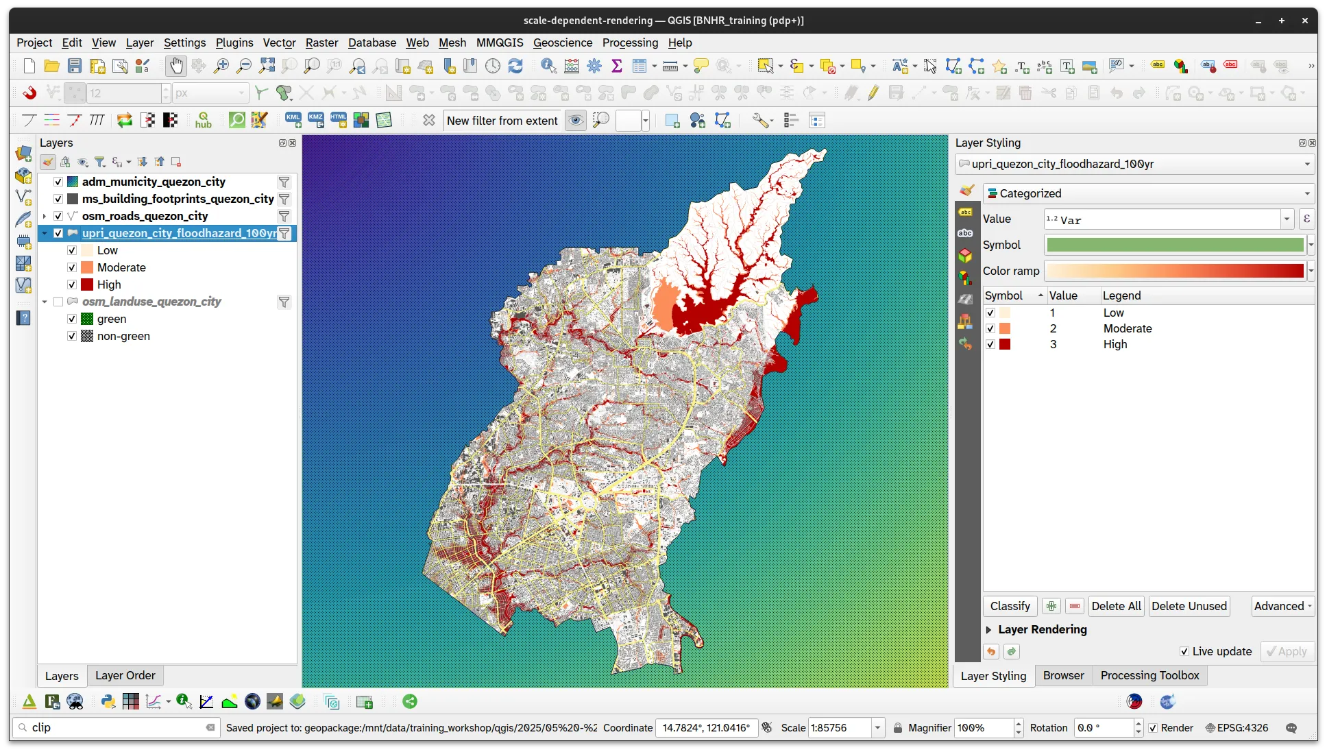
- Load the upri_quezon_city_floodhazard_100yr and ms_building_footprints_quezon_city layers and style them accordingly.
-
For osm_roads_quezon_city, set the following parameters for the others rule:
- Min. Scale:
1:50000 - Max. Scale:
1:1
Don’t forget to apply your changes.
- Min. Scale:
- Do the same for the non-green rule in osm_landuse_quezon_city but with the following parameters:
- Min. Scale:
1:10000000 - Max. Scale:
1:25000
- Min. Scale:
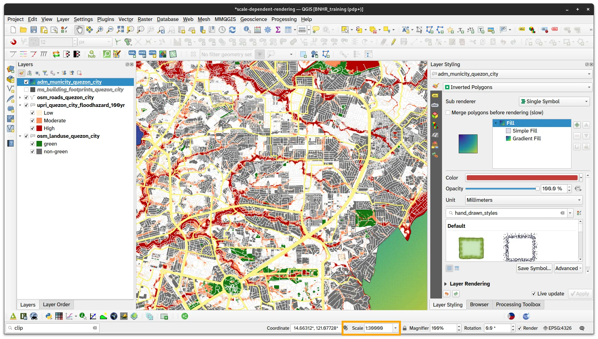
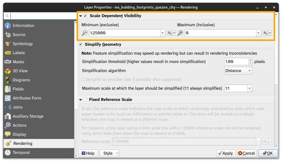
- For upri_quezon_city_floodhazard_100yr, open its Layer Properties and go to the Rendering tab. Check the Scale Dependent Visibility and put
1:50,000as the Minimum.
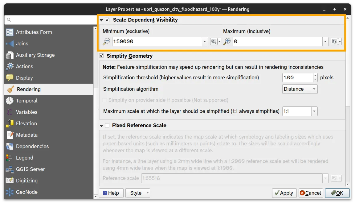
- Look at your map canvas. You should notice that when you are zoomed out (or when the scale is less than 1:50,000), the other roads and the flood hazard are not visible and when you zoom in (or once the scale is greater than 1:50,000) they appear.
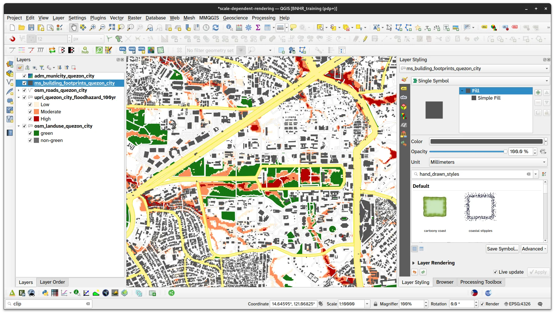
- For ms_building_footprints_quezon_city, do the same thing that you did for upri_quezon_city_floodhazard_100yr but put the Minimum to
1:25,000.
Take a look at you map canvas again, this time the building data should only appear when the scale is greater than 1:25,000.
Certification and support
Section titled “Certification and support”Contact us or sign-up to our courses if you are interested in having this as an instructor-led or self-paced course.