
All about data
Introduction
Section titled “Introduction”This module discusses tips, tricks, caveats, and gotchas when working with geospatial data in QGIS.
What you should already know
Section titled “What you should already know”As a foundational module, no previous knowledge of GIS or QGIS is required. However, familiarity with the QGIS interface as discussed in QGIS: Essentials - Introduction to QGIS, how to load different kinds of layers as discussed in QGIS: Essentials - Introduction to layers in QGIS, and how to run processing algorithms as discussed in QGIS: Essentials - Basic geospatial processing techniques are preferred.
Where to find free and open geospatial data
Section titled “Where to find free and open geospatial data”Plugins that help you access/download data directly in QGIS
Section titled “Plugins that help you access/download data directly in QGIS”Some of the most common and useful QGIS plugins are those that allow you to directly download data in QGIS. Some of these plugin include:
QuickOSM plugin
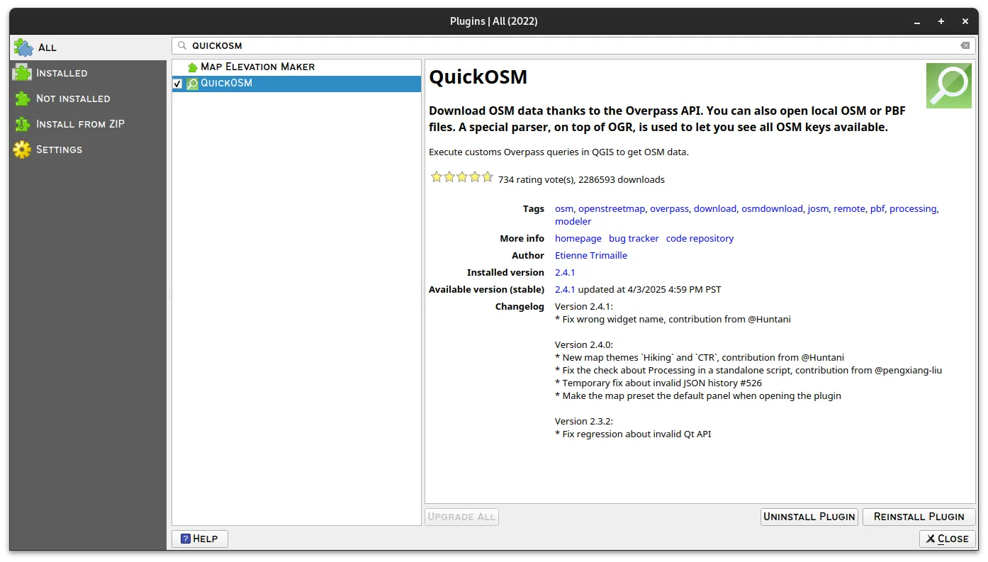
Section titled “QuickOSM plugin”The QuickOSM plugin allows you to “download OSM data thanks to the Overpass API. You can also open local OSM or PBF files. A special parser, on top of OGR, is used to let you see all OSM keys available.”
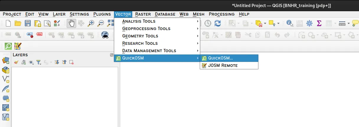
Once installed and activated, the plugin can be run from the main menu under Vector ▸ QuickOSM ▸ QuickOSM
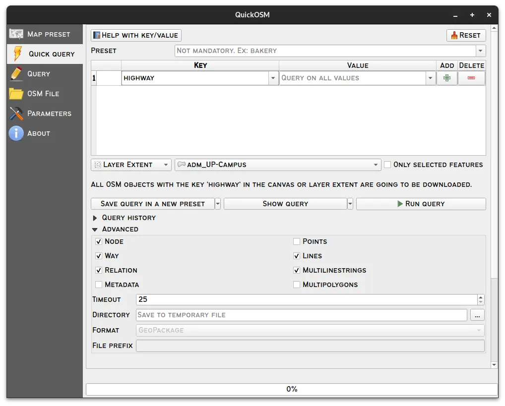
This will open the QuickOSM window. The easiest way to download data using QuickOSM is via the Quick Query tab and providing:
- Key
- Value
- Extent
- Other Advanced Parameters
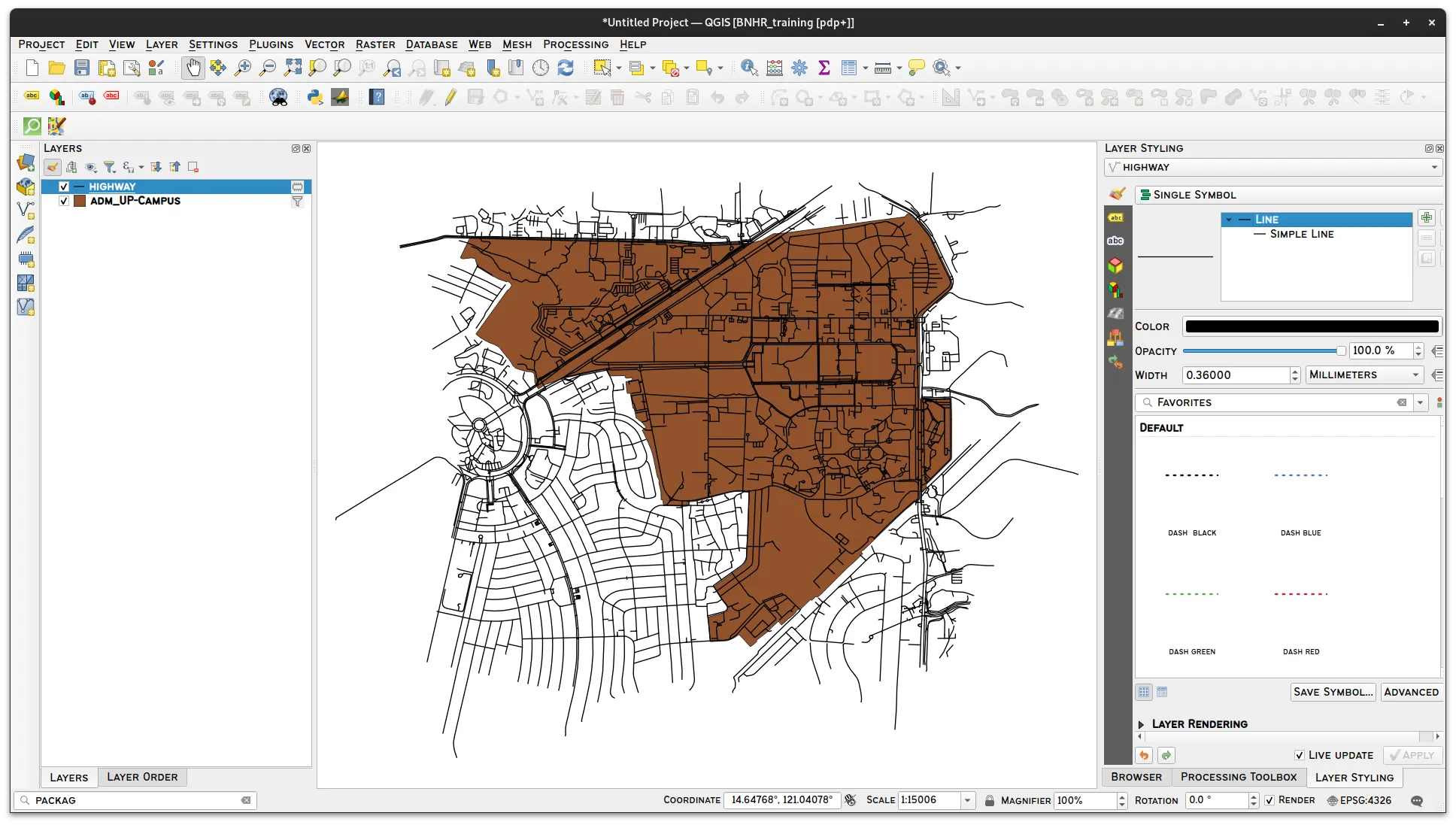
For example, if we want to download all linear vector data for roads (key on OSM is highway) within Barangay UP Campus, we can provide the following parameters:
- Key: highway
- Value: blank (means all values)
- Extent: Layer Extent (adm_UP_Campus or whatever layer we want to use)
- Advanced:
- check Lines, Multilinestrings
After we click Run Query, the plugin will try to load all data from OSM that meet the criteria we set.
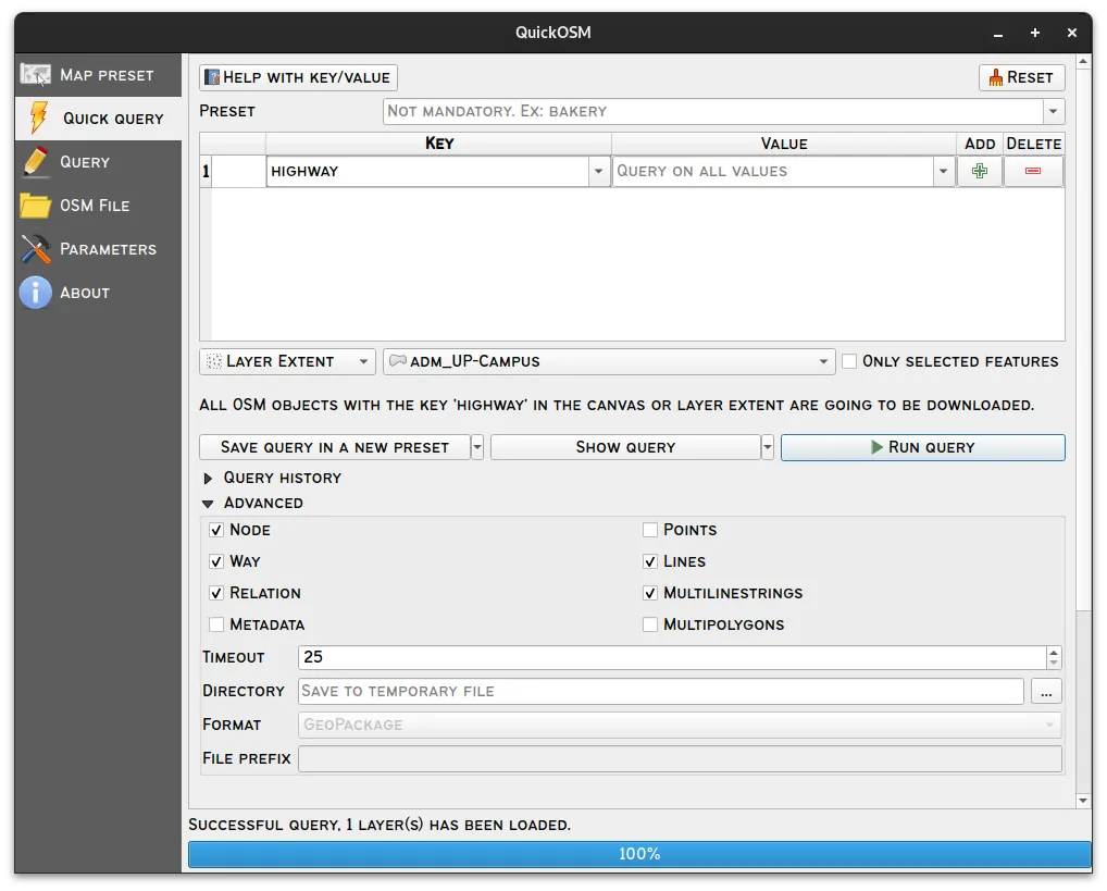
You will see that a highway layer is loaded after running the query in QuickOSM.
There are other ways to use QuickOSM to load data in QGIS. To learn more, you can read its documentation or watch below:
OpenTopography DEM Downloader plugin
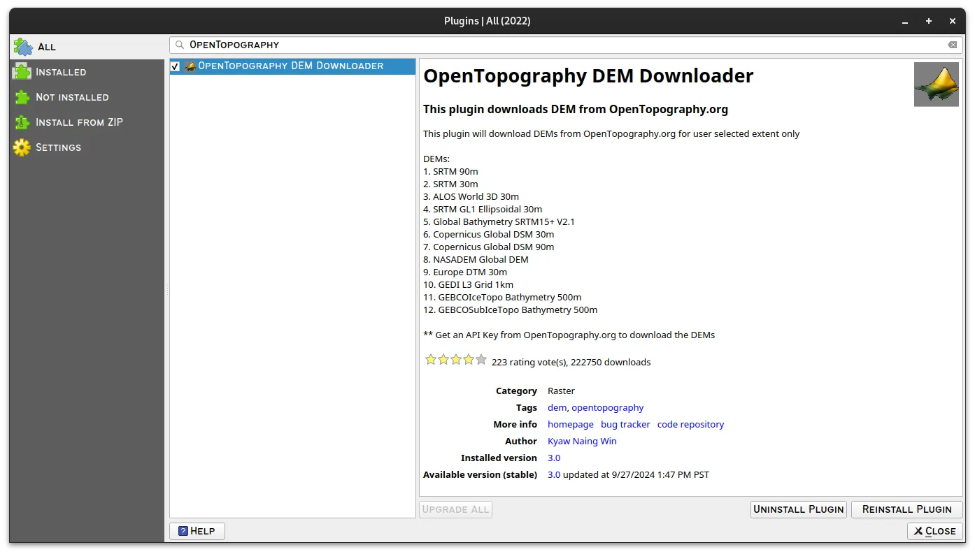
Section titled “OpenTopography DEM Downloader plugin”The OpenTopography DEM Downloader will “download DEMs from OpenTopography.org for user selected extent only.”
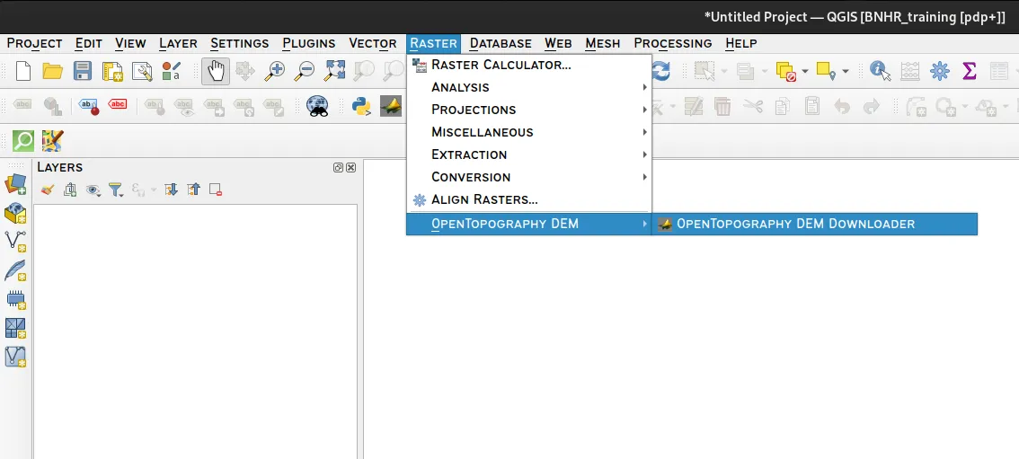
Once installed and activated, the plugin can be run from the main menu under Raster ▸ Open Topography DEM ▸ OpenTopography DEM Downloader
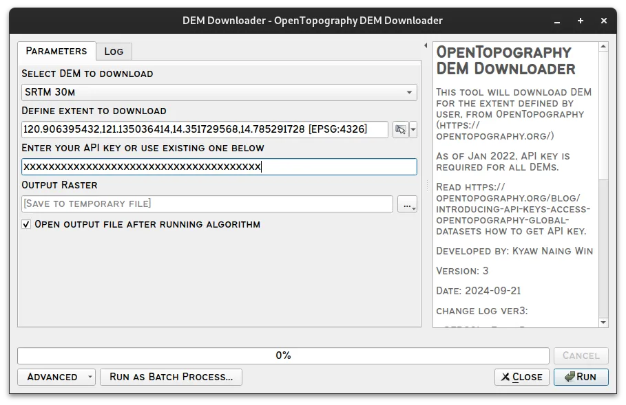
This will open the OpenTopography DEM Downloader window where you can specify the:
- DEM you want to download
- Extent you want to download
- API key
- Output raster
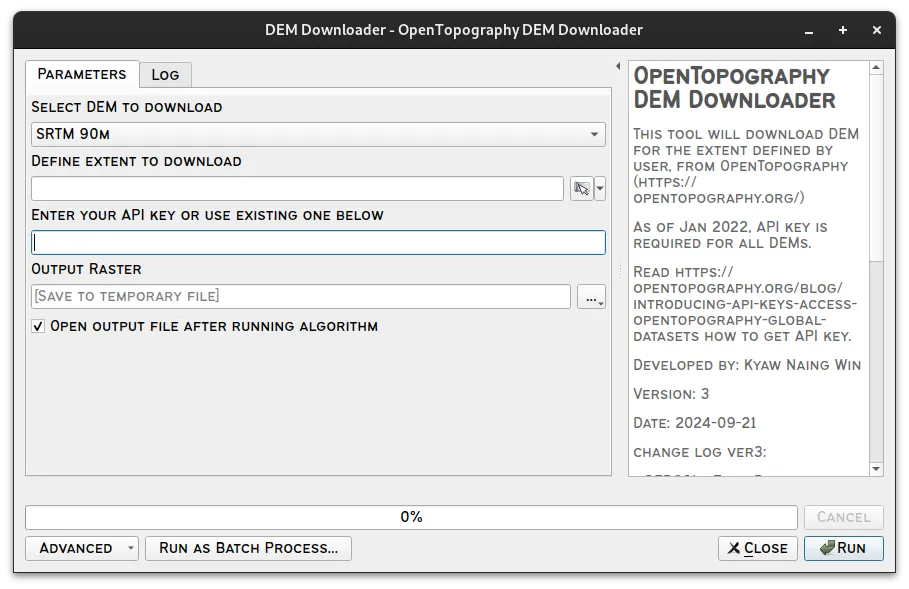
For example, if we want to download an SRTM 30m DEM covering the extent of the National Capital Region, we will provide the following parameters:
- DEM: SRTM 30m
- Define extent to download: Calculate from Layer > adm_NCR (or whatever layer we want to use)
- Enter your API key or use existing one below: the API key you generated with your OpenTopography account
You will see that an SRTMGL1[memory] raster layer is loaded after successfully running the OpenTopography DEM Downloader plugin.
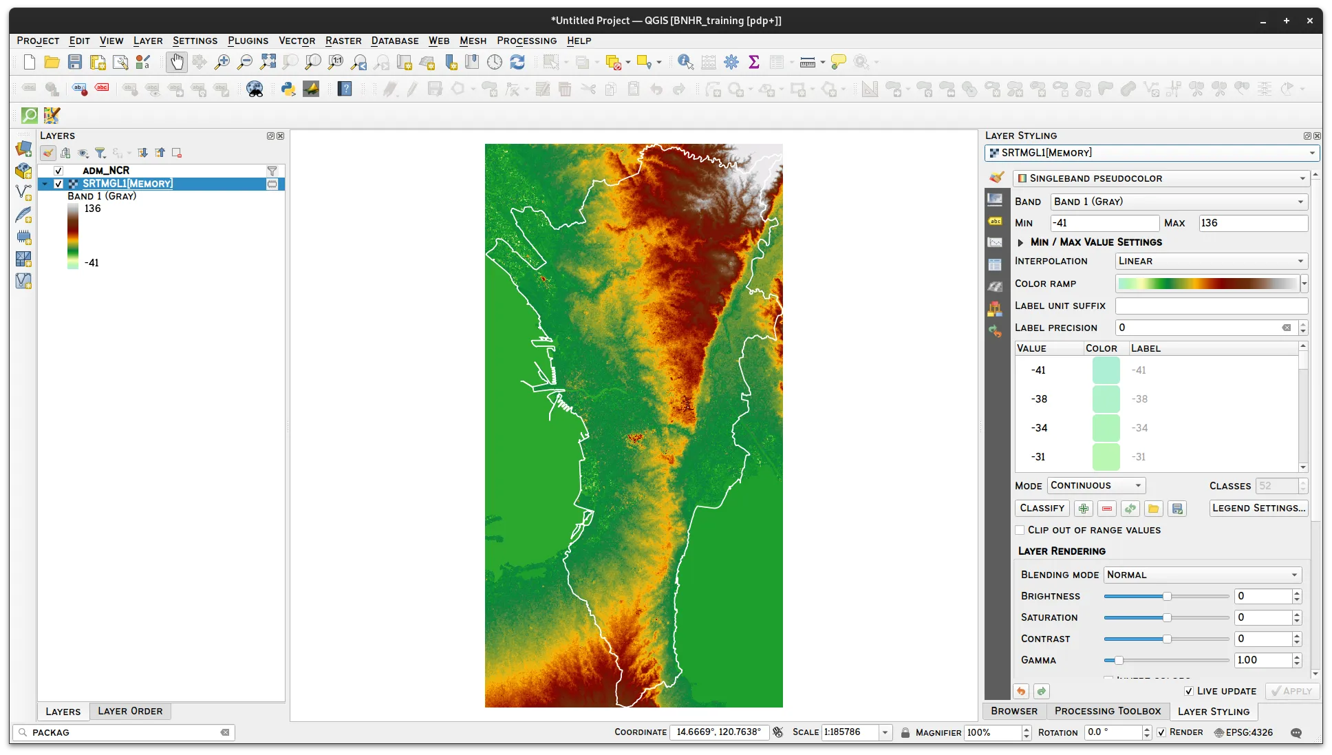
You can use this layer as you would any raster layer in QGIS but take note that it is still a temporary layer so you need to save it in order to make it persistent.
STAC API Browser
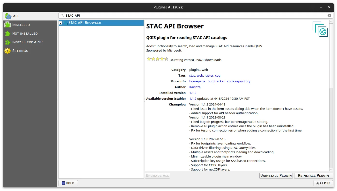
Section titled “STAC API Browser”The STAC API Browser plugin “adds functionality to search, load and manage STAC API resources inside QGIS.”
STAC or the SpatioTemporal Asset Catalog is a family of specifications designed to help standardize the way collections of geospatial (and temporal) data are exposed, structured, and queried. In other words, it makes it easy to catalog, search, and load geospatial data.
Once installed and activated, the plugin can be run from the main menu under Plugins ▸ STAC API Browser Plugin ▸ Open STAC API Browser.
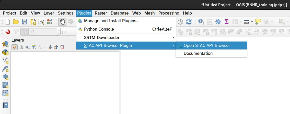
This will open the STAC API Browser window where you can search for data given the following parameters:
- Connections: the STAC API to use
- Collections: the STAC collections available in the Connection
- Filters: ability to filter the collections/data to search
- Date
- Extent
- Other advanced filters
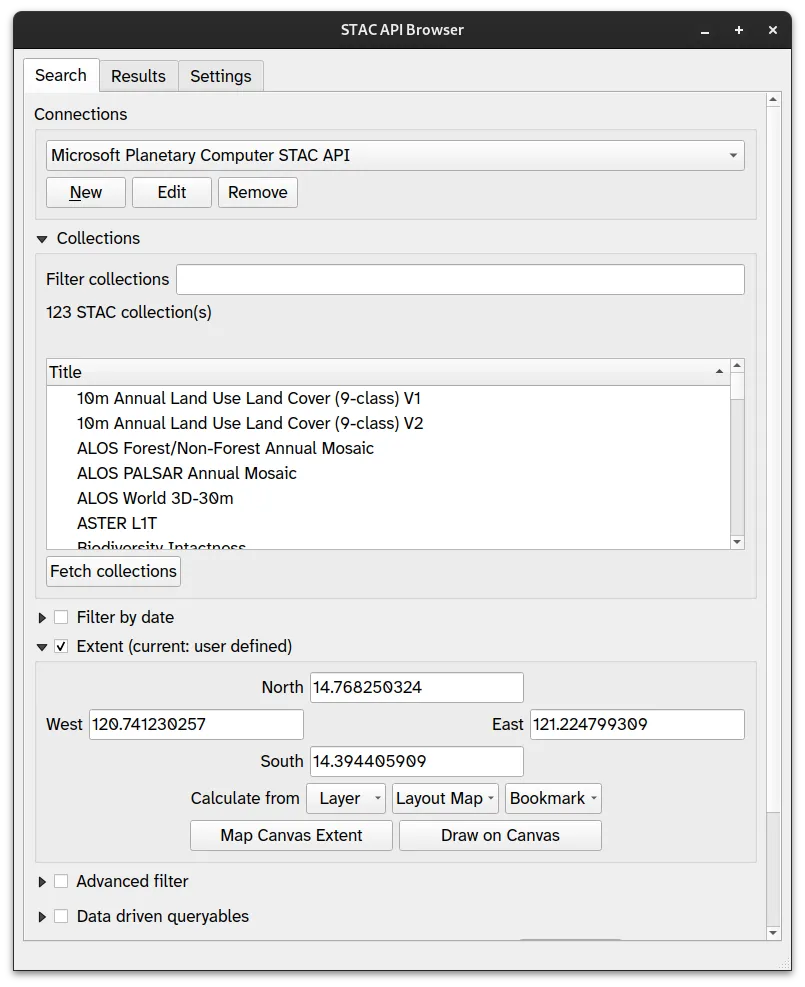
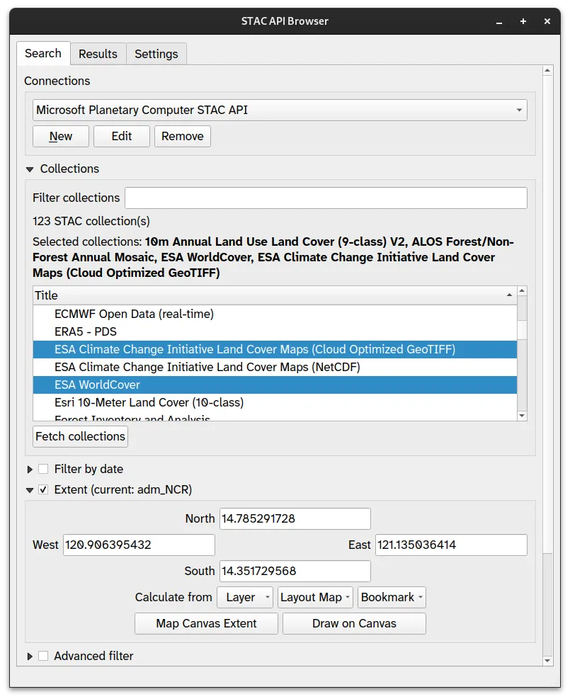
For example, if we want to search for Land Use/Land Cover-related data for NCR from the Microsoft Planetary Computer STAC API, we may want to use the following parameters:
- Connections: Microsoft Planetary Computer STAC API
- Collections:
- 10m Annual Land Use Land COver (9-class) V2
- ESA Land Cover
- ESA WorldCOver
- ESA Climate Change Land Cover Maps (Cloud Optimized GeoTIFF)
- Extent:
- Calculate from Layer (adm_NCR or any layer we want to use)
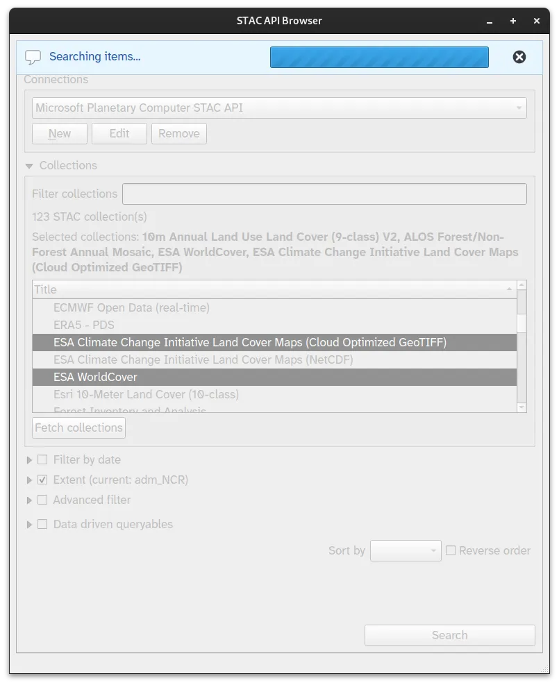
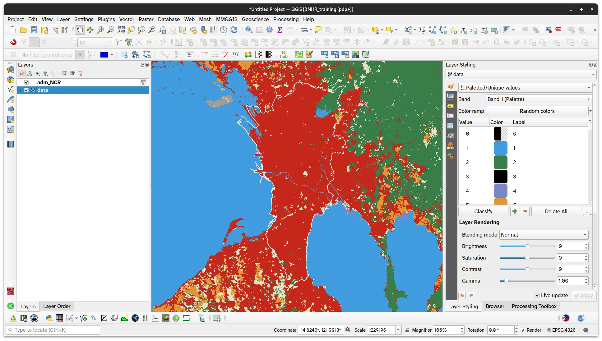
Clicking Search will search for data in the selected collections that include our provided extent (NCR).
Once the Search is completed, we can find all the available data in the Results tab.
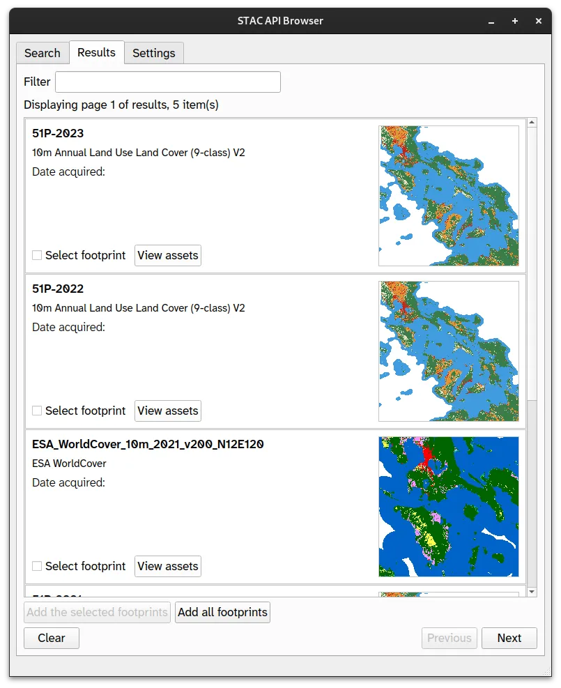
To load the data in QGIS, click on View Assets to open the Assets window. Check Select to add as layer then click Add selected assets as layers.
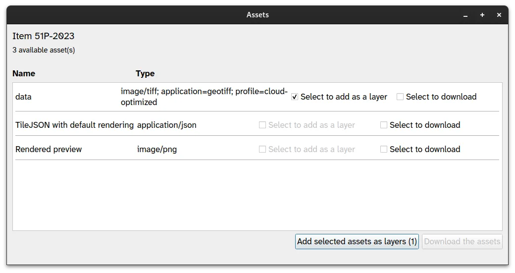
The selected asset will then be loaded in QGIS.
To learn more about the plugin, visit its documentation
External sources, data portals, etc.
Section titled “External sources, data portals, etc.”There exists countless data sources online where you can find and download geospatial data—from data portals, web services, APIs, and websites hosting data. Some examples are:
- Awesome Data Philippines (https://bnhr.xyz/awesome-data-philippines/)
- Philippine Geoportal (http://www.geoportal.gov.ph/)
- Open Data Philippines (https://data.gov.ph/)
- Project NOAH/UP Resilience Institute (https://drive.google.com/drive/folders/1ALE4-E9c-4AGjm1fqiPprWHrLUskeY9o)
- Philippines Statistics Authority Data Archive (http://psada.psa.gov.ph/index.php/home)
- USGS Earth Explorer (https://earthexplorer.usgs.gov/)
- NASA Earthdata Search (https://search.earthdata.nasa.gov/search)
- Registry of Open Data on AWS (https://registry.opendata.aws/)
- Awesome Google Earth Engine Community Catalog (https://gee-community-catalog.org/)
- And many more…
To work with these data sources in QGIS, it is imperative that you know how to load diffirent kinds of data or how to connect to different services in QGIS.
Not all data are created equal
Section titled “Not all data are created equal”The fault in our administrative boundary data
Section titled “The fault in our administrative boundary data”Administrative boundary data is a core dataset frequently used in any mapping or GIS activity. In the Philippines, they typically come from two common sources:
- GADM (https://gadm.org/download_country.html)
- Humanitarian Data Exchange via OCHA, PSA, and NAMRIA (https://data.humdata.org/dataset/cod-ab-phl)
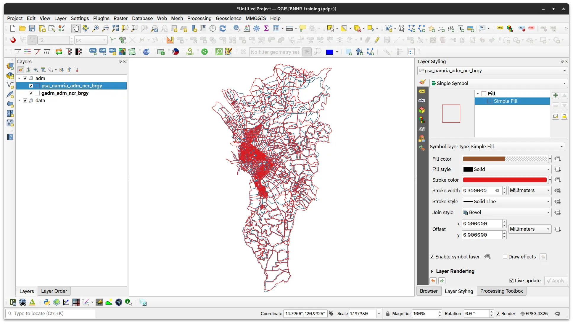
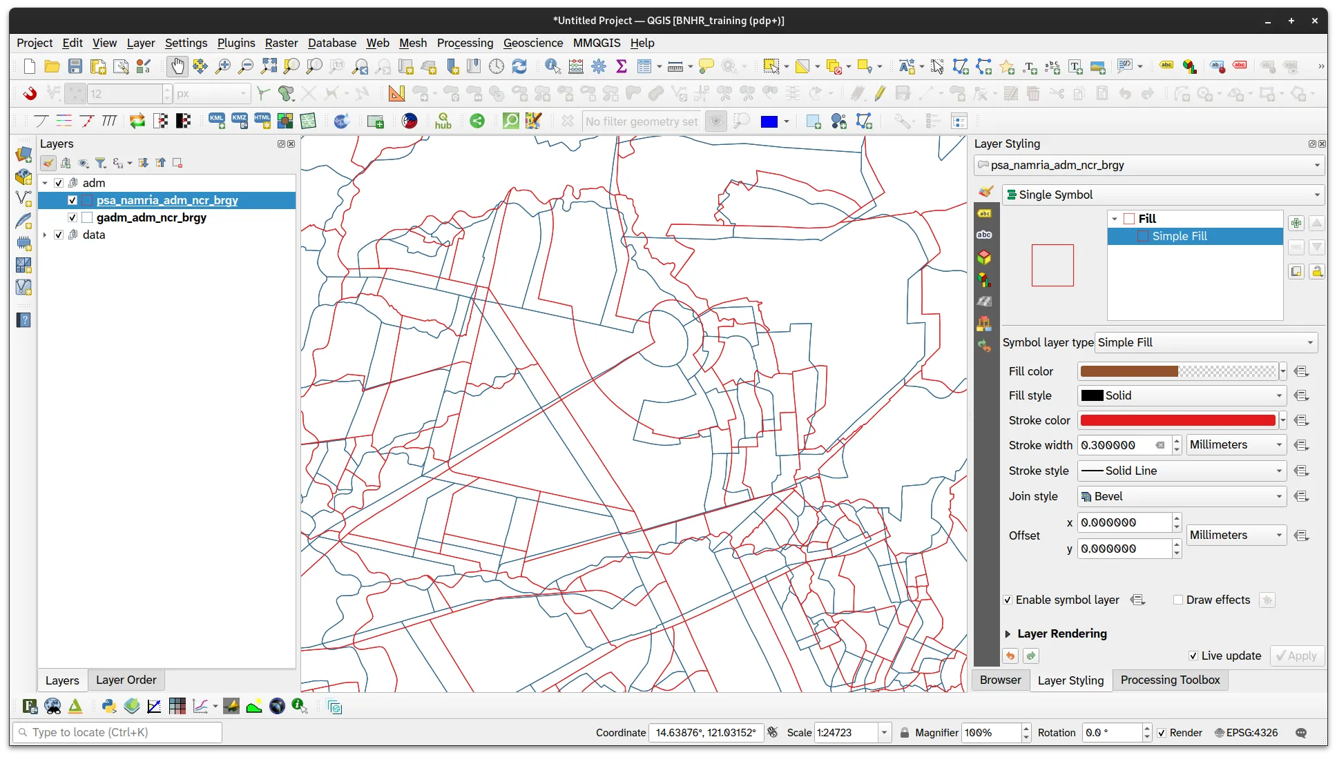
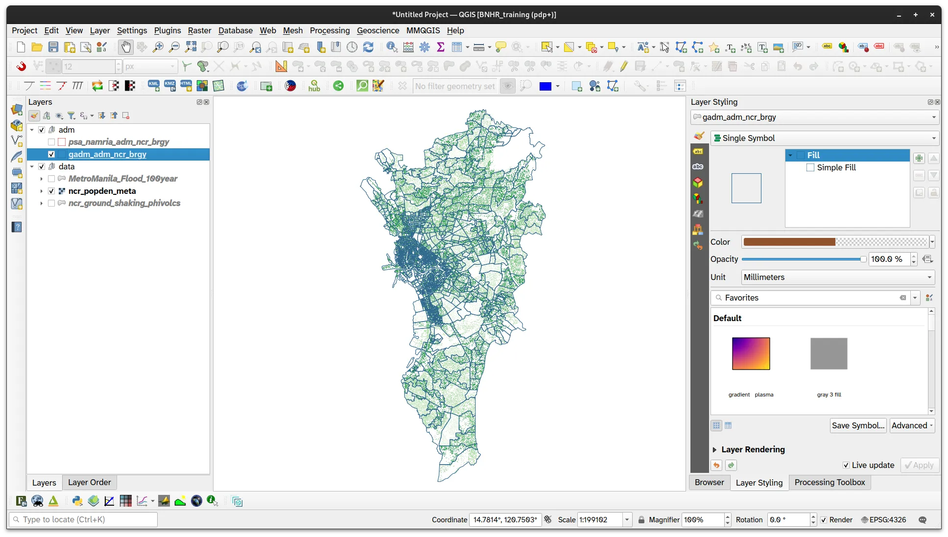
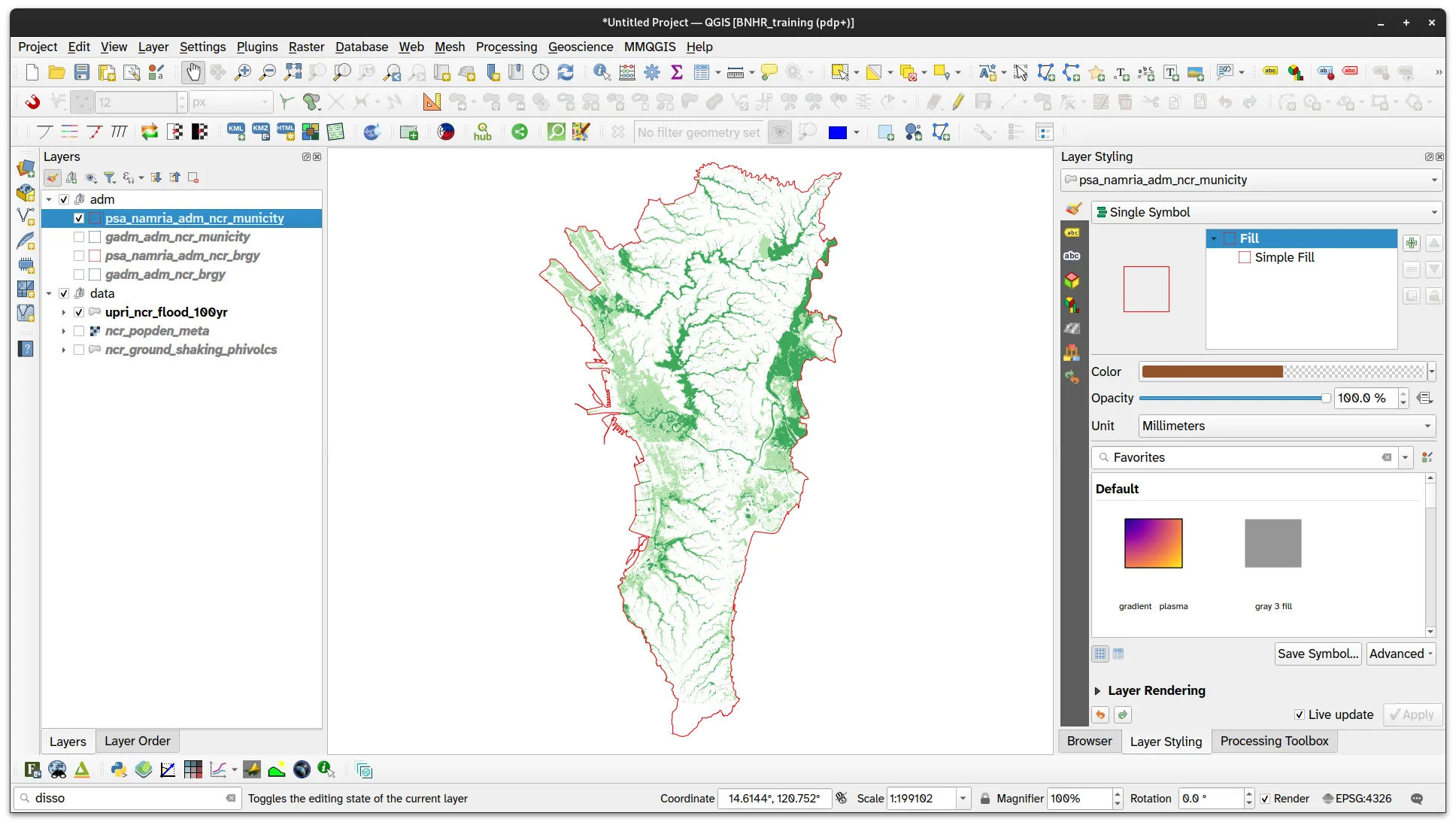
If you look at the barangay boundary data of the layers from these two sources, you will notice that they are not equal and, in fact, there are significant differnces in the shapes and areas of the barangays. This is important because these differences will reflect in the mapping and GIS activities done using these datasets.
The propagation of errors
Section titled “The propagation of errors”Other data that rely on administrative boundaries (e.g. to clip or subdivide the data) must make a choice as to what admin boundary data to use and—as mentioned above—this choice affects the final dataset.
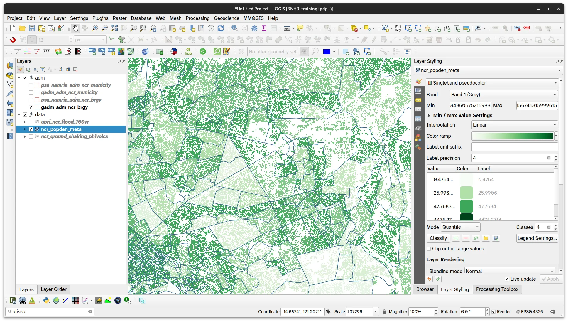
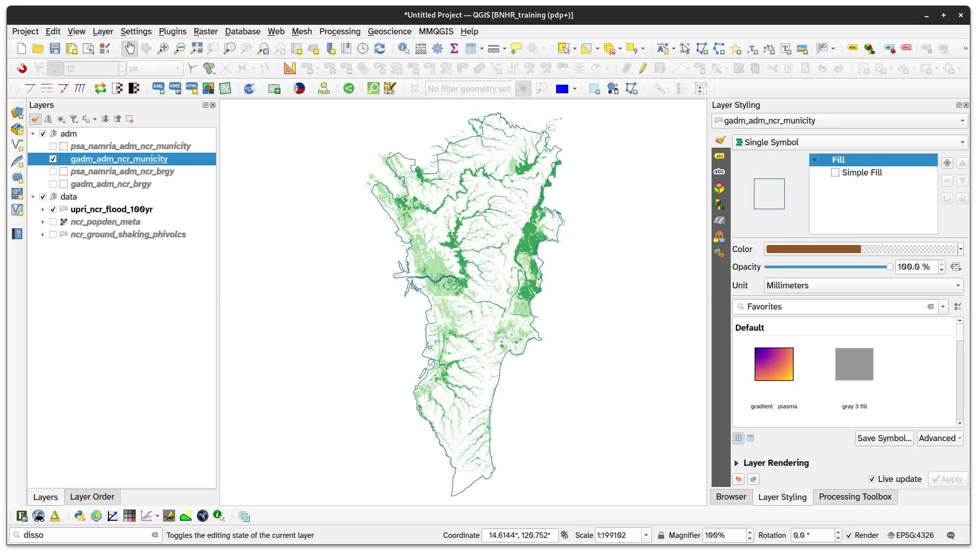
For example, if you look at Meta’s High Resolution Population Density Maps, it becomes clear that they used GADM.
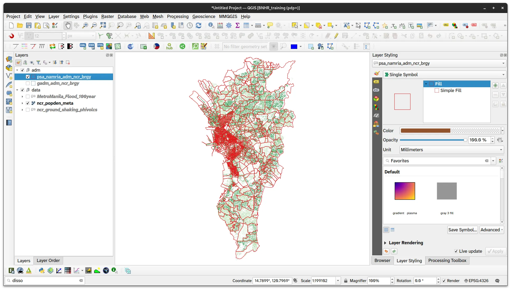
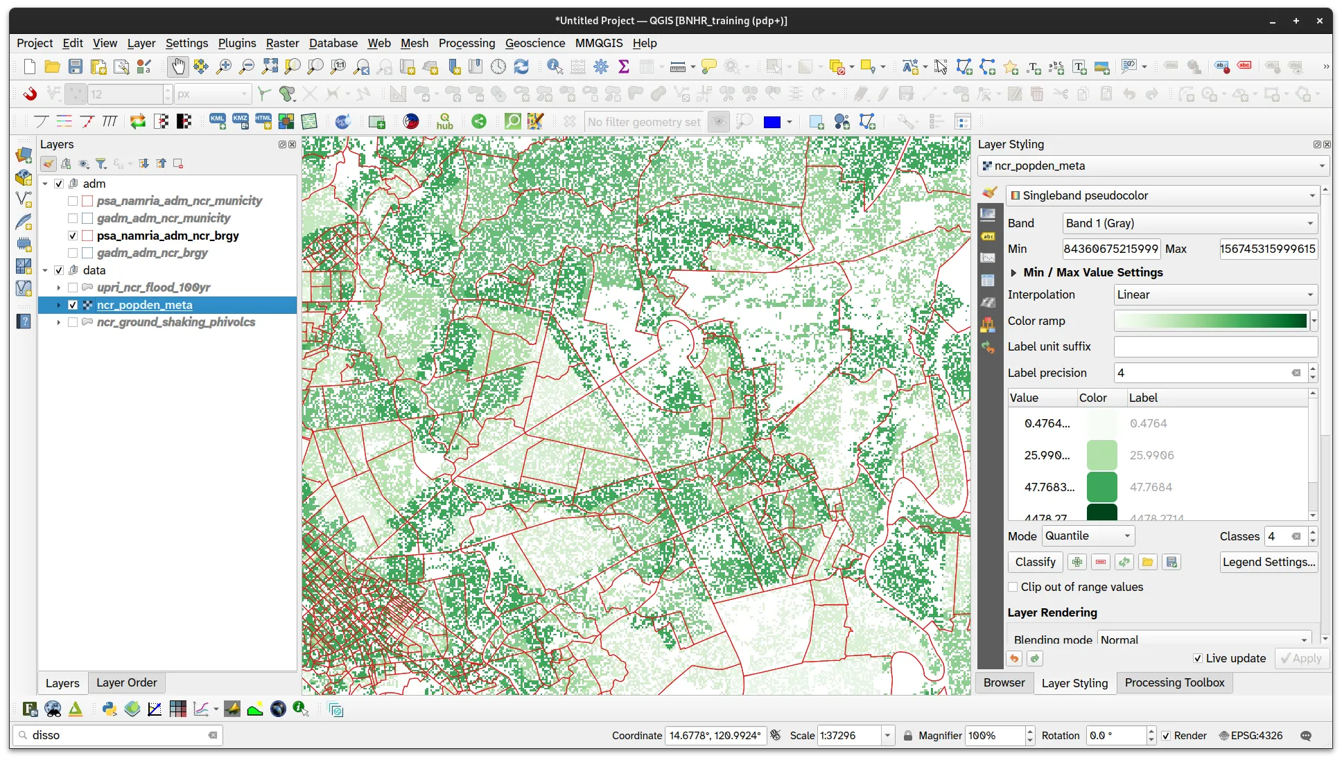
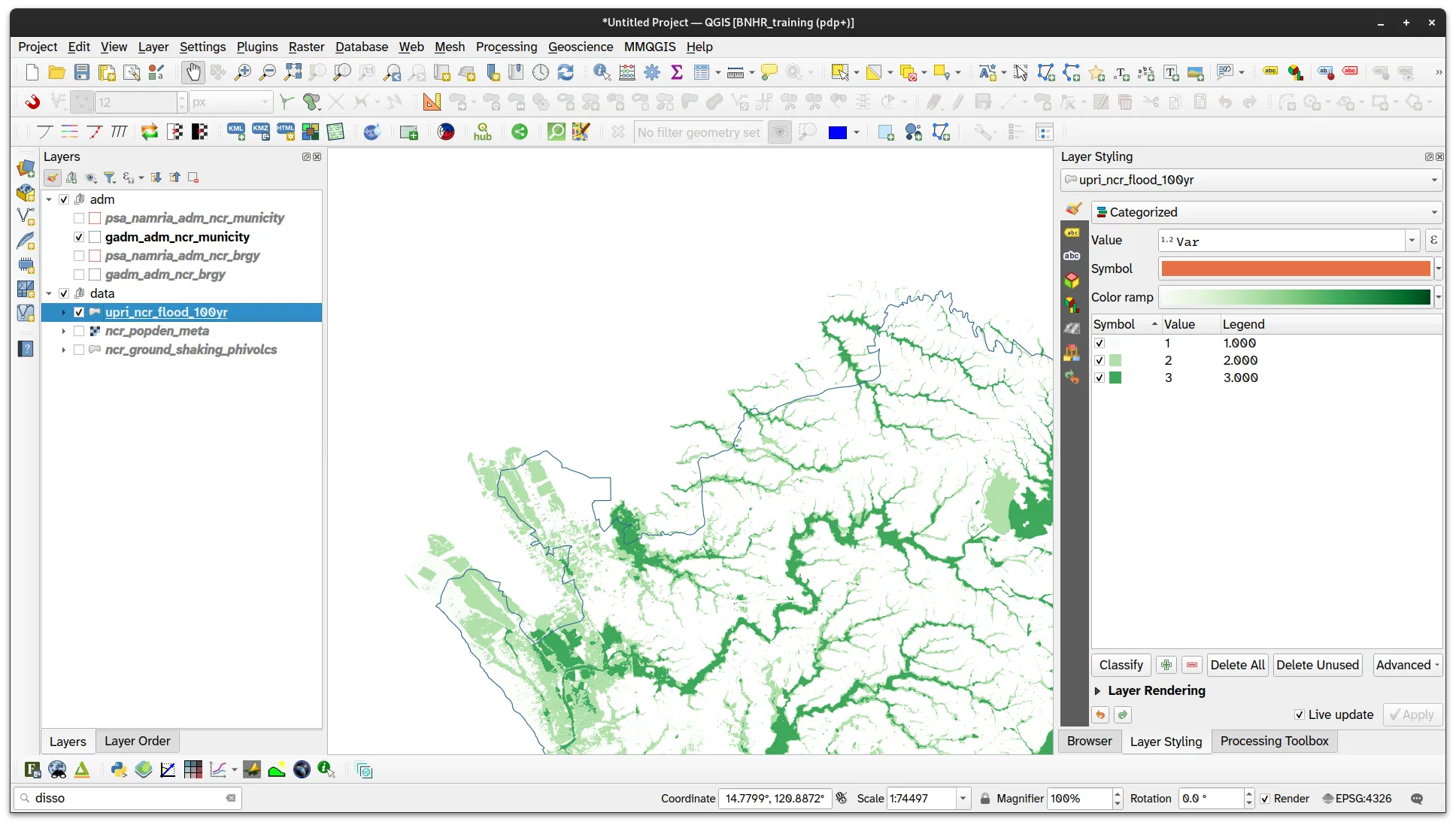
On the other hand, if you look at Project NOAH/UP Resilience Institute’s Flood Hazard data, you will notice that the flood layer was clipped using the HDX UN OCHA/PSA/NAMRIA layer.

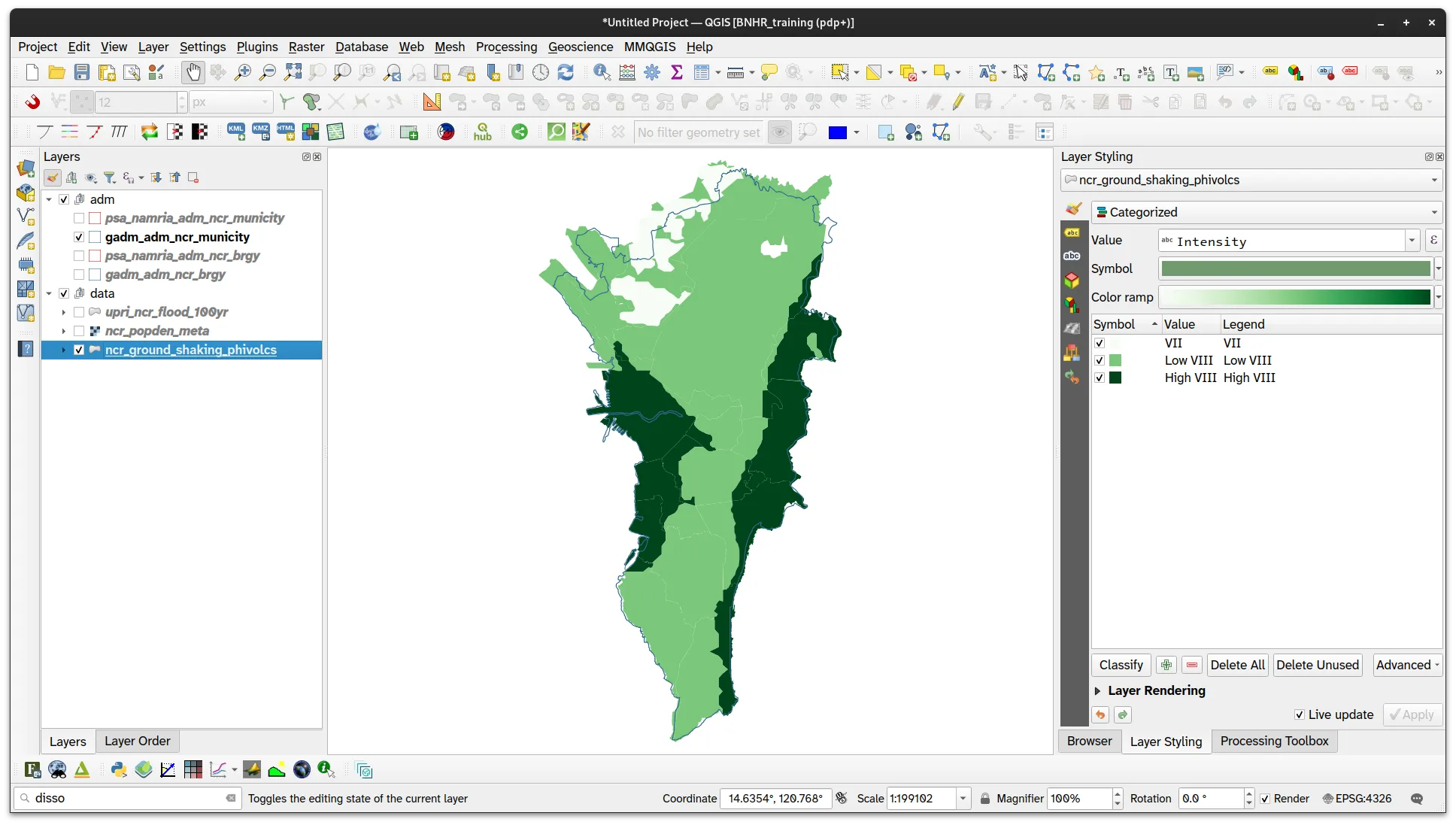
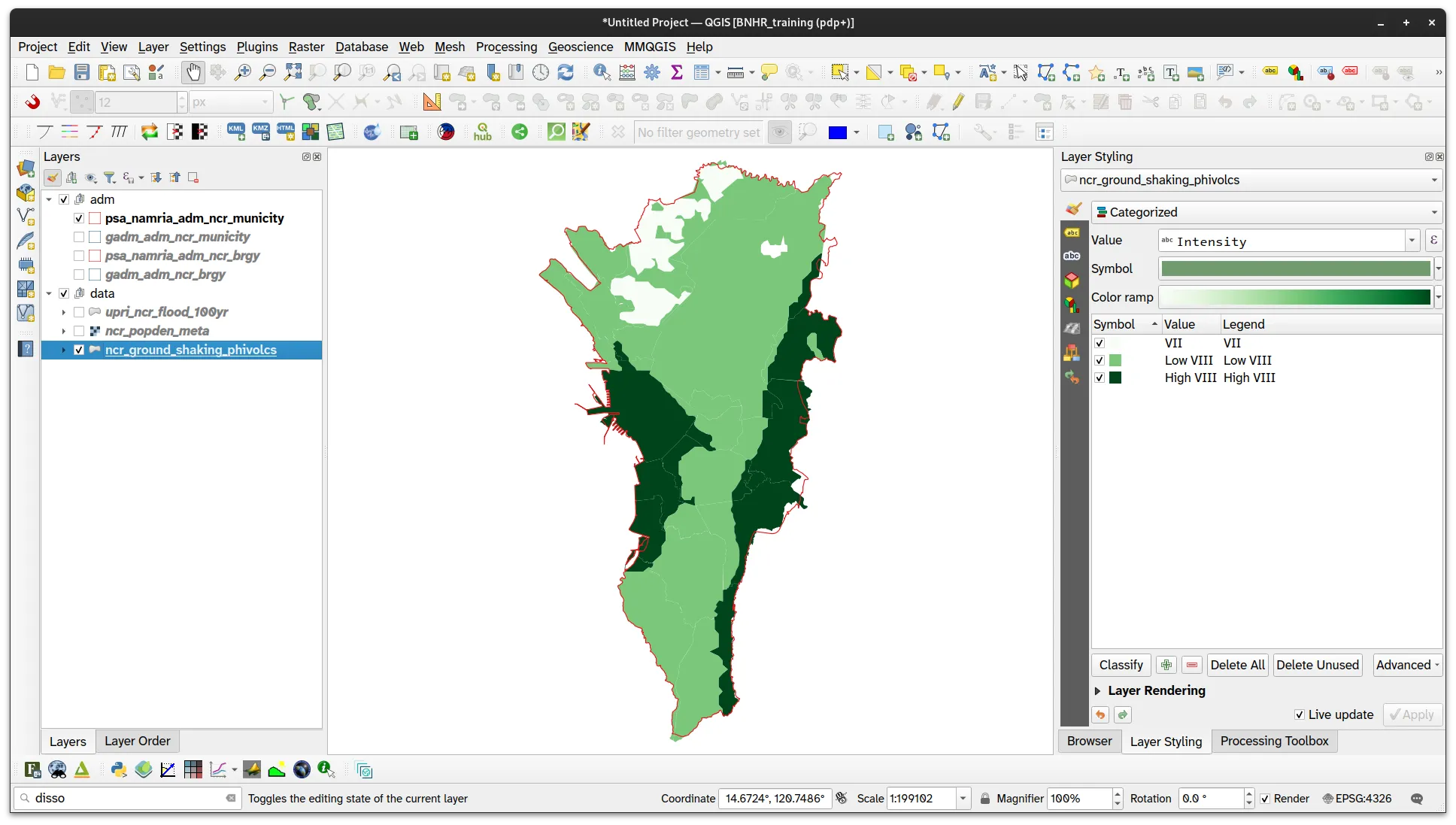
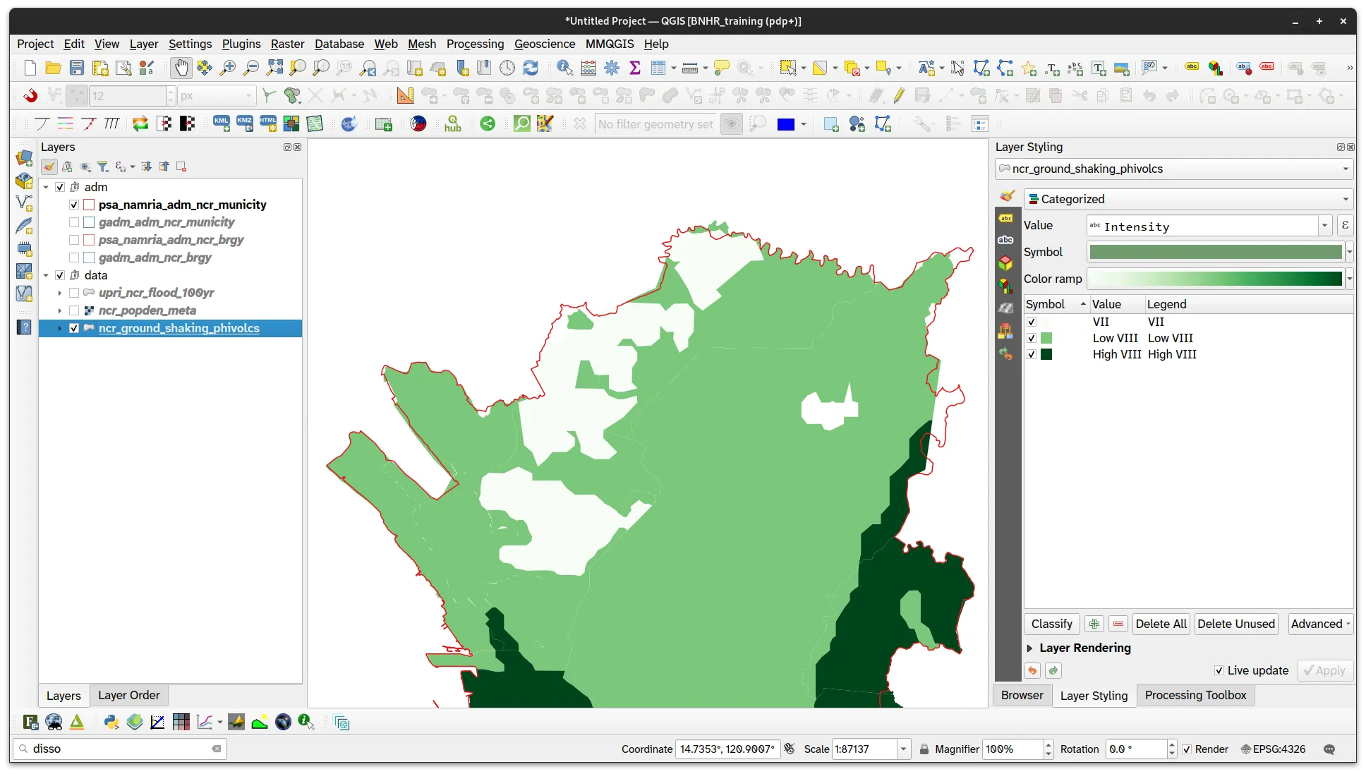
And then there are those that do not conform to any of the two common admin boundary data. For example: if you look at the Ground Shaking Hazard from PHIVOLCS, it does not align perfectly with either the GADM or the HDX (UN OCHA/PSA/NAMRIA) NCR admin boundary.

Certification and support
Section titled “Certification and support”Contact us or sign-up to our courses if you are interested in having this as an instructor-led or self-paced course.