Making data usable in QGIS

Introduction

In this module, you will be introduced to different processes of preparing and formatting data so that it can be loaded and analyzed in QGIS or in any geospatial application.

At the end of this module, you should know what to do if: you have a spreadsheet or CSV file with coordinates, you have a PDF/image of tabular data with coordinates, you have a spreadsheet or CSV file that doesn’t have coordinates but has a column pertaining to its location, you have have an image of an area but it doesn’t load in the correct location in QGIS, you want to create a new layer, or you have an image or map and you need to extract information from it.

What you should already know

Since this is a beginner module, no previous knowledge of GIS or QGIS is required. However, familiarity with the QGIS interface as discussed in QGIS: Essentials - Introduction to QGIS, how to load different kinds of layers as discussed in QGIS: Essentials - Introduction to layers in QGIS, and how to run processing algorithms as discussed in QGIS: Essentials - Basic geospatial processing techniques are preferred.

Making data usable in QGIS

Geospatial data is an essential and ubiquitous component of modern life—powering everything from navigation apps to climate modeling. This is why it is crucial to have the tools and skills to work with a variety of data formats. While some of these data formats may be readily available in digital form that can easily be loaded and used in QGIS or other geospatial applications, there are many instances when it is not.

Often, data comes in a format that is not immediately usable in GIS software like QGIS. Or, even when data is in a usable format, it may be geographically displaced or incomplete, requiring additional steps to bring it into a usable form. This is why working with data (especially geospatial data) can be a challenging task.

The goal of this module is to provide you with a guide to making data usable in QGIS. Whether you are working with spreadsheets, images, or maps, the techniques covered in this module will help you prepare, process, and format your data so that it can be loaded into QGIS and used to create accurate, informative, and impactful geospatial analyses and visualizations.

Each chapter of this workbook focuses on a different scenario you may encounter when working with geospatial data and provides step-by-step guidance on how to handle these situations. From spreadsheets with coordinates to digital images that need to be georeferenced, this module covers most of the things you need to know to make your data usable in QGIS.

With the knowledge and techniques presented in this module, you will be able to turn raw geospatial data into powerful and informative outputs no matter what project you’re doing.

What to do when: you have a file or table with coordinates

LEARNING OBJECTIVES

1. Understand how to import files or tables with coordinate data into QGIS.
2. Understand how to handle coordinate systems and projections.
3. Gain hands-on experience importing and working with data in QGIS.

CSVs, spreadsheets, and PDFs are commonly used formats for storing and presenting data. Sometimes they contain location data in the form of latitude and longitude coordinates, address information, place names, or sometimes even actual geometries (e.g. WKT or Well-Known Text).

It is important to understand what to do in order to load a CSV, spreadsheet, or PDF with location information as a geospatial layer in QGIS.

Examples when you will encounter this scenario include:

1. Using geotagged surveys/data exported from field data collection applications like ODK and Kobo Toolbox.
2. Getting location information from PDF reports.

Spreadsheets or CSVs with coordinates

QGIS allows you to easily load CSVs and other delimited text files via the Data Source Manager and spreadsheets using the Spreadsheet Layers plugin.

Recall: Loading delimited text files and spreadsheets in Essentials

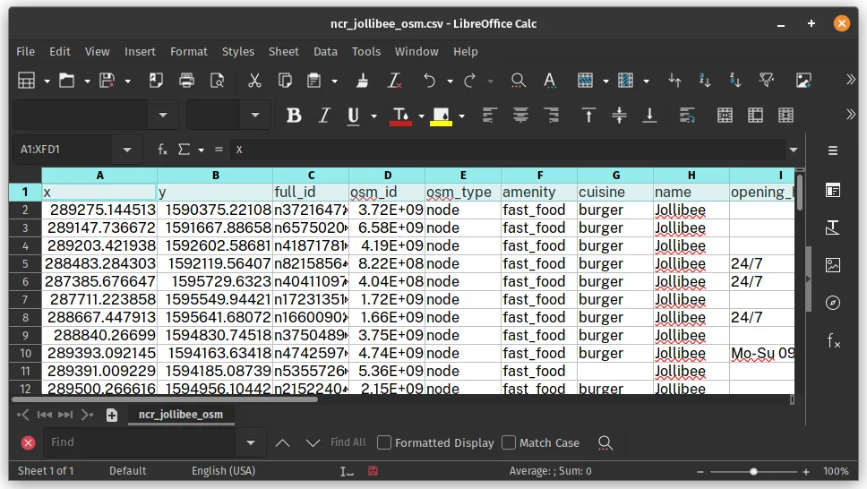
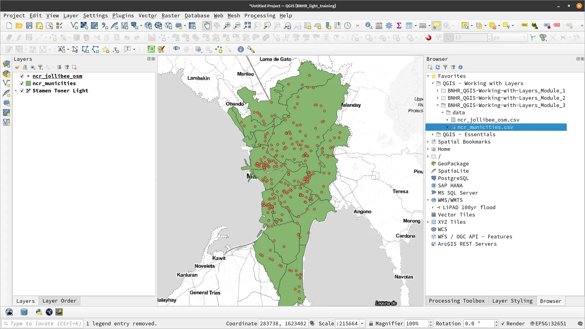
Exercise 3.1. Loading some more CSV files

In this exercise, we will load two more CSV files—ncr_jollibee_osm and ncr_municities—that are a bit different than the ones in the Essentials workbook.

1. Let’s start with ncr_jollibee_osm. Open the CSV in a text editor or spreadsheet of your choice. What fields can we use for coordinates? What are their values

Figure 1. ncr_jollibe_osm CSV

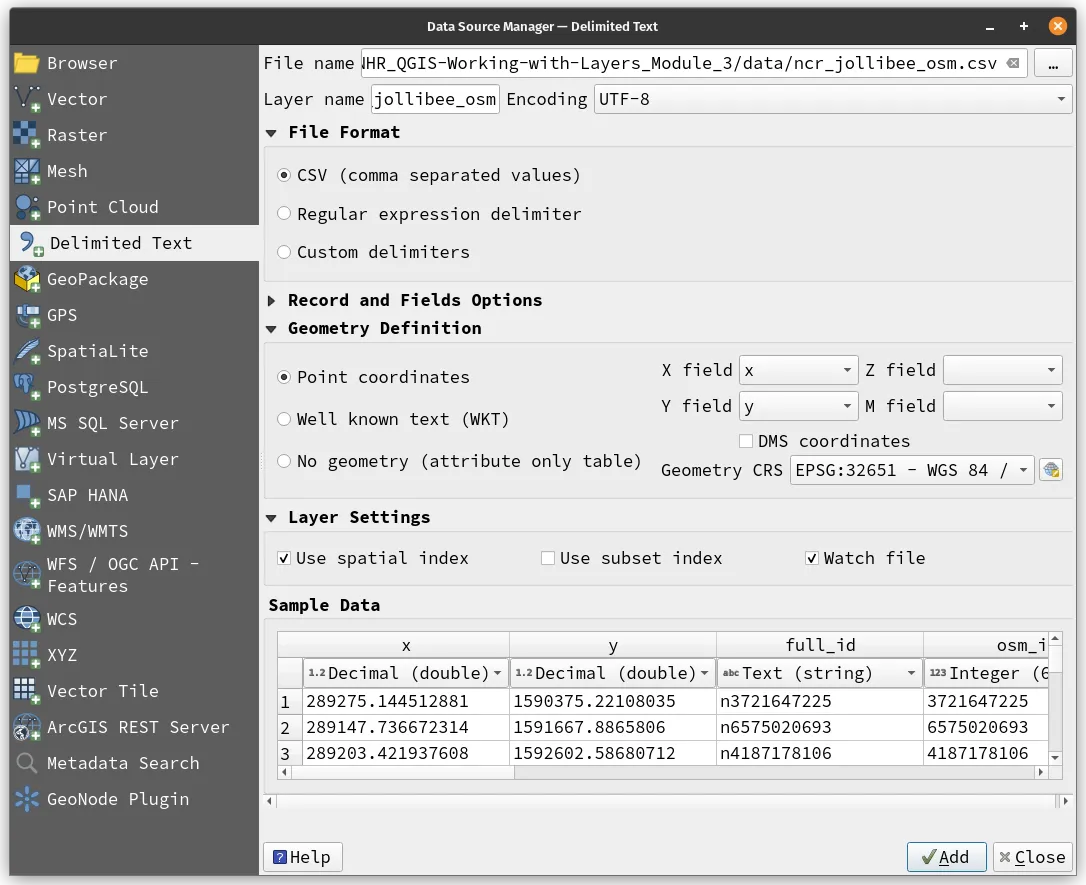
2. Open the Data Source Manager and go to the Delimited Text tab.
3. Use the following parameters to load the CSV.
   • File format: CSV
   • Geometry definition: Point coordinates
     • X field: x
     • Y field: y
   • Geometry CRS: EPSG:32651

Figure 2. Parameters for loading the ncr_jollibe_osm CSV

SOMETHING TO THINK ABOUT

What’s different about this compared to the one we loaded in Essentials?

PRO-TIP

It is important to keep in mind the CRS used by the coordinates in our CSVs or spreadsheets. Using an incorrect CRS will load your data in the incorrect location or not load it at all.

Always make sure that you are using the correct CRS when loading your delimited text files or spreadsheets.

Figure 3. ncr_jollibee_osm CSV loaded in QGIS

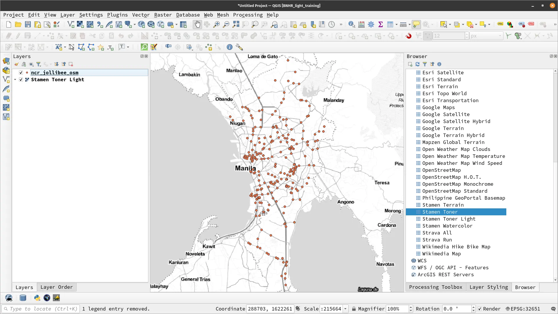
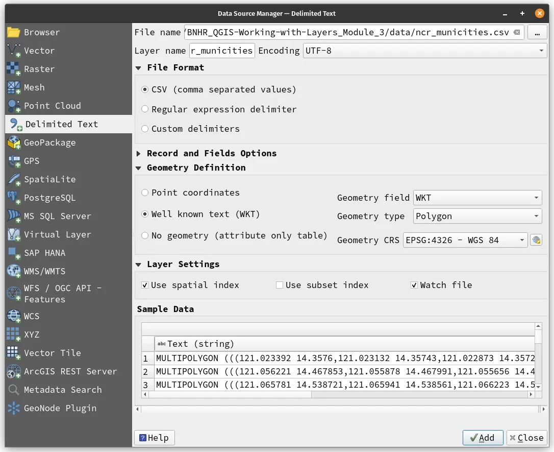
4. Now let’s try the ncr_municities CSV. What’s different with this CSV is that it doesn’t hold point data but polygon features. If you open the CSV, you will find a field/column that named WKT that includes values that say POLYGON… These values are the Well-Known Text representation of the feature and can be read by geospatial applicatons such as QGIS to load the feature/geometry.

PRO-TIP

It isn’t just point coordinates that you can load via CSV in QGIS. A CSV can be of any geometry by using a field that uses values such as WKT or Well Known Text.

5. Use the following parameters to load the CSV.
   • File format: CSV
   • Geometry definition: Well known text (WKT)
   • Geometry CRS: EPSG:4326

Figure 4. Parameters for loading the ncr_municities CSV

6. It should be loaded like below.

Figure 5. All CSV layers loaded in QGIS

About Well-Known Text (WKT)

Well-Known Text (WKT) is a text format used to represent vector geometry objects in GIS. It is a standardized way of describing geometry types such as points, lines, polygons, and multi-geometries, using a human-readable text string.

WKT is useful because it allows geometry data to be shared between different GIS software, even if they are based on different platforms or programming languages. It is also used as an input format for certain spatial databases and programming libraries.

It follows a specific syntax with each geometry type having its own format. For example:

• a point geometry is represented as “POINT (x y)” where x and y are the coordinates of the point.
• a line geometry is represented as “LINESTRING (x1 y1, x2 y2, … xn yn)” where each pair of x and y values represents a point on the line.

PDF/image of tabular data with coordinates

Sometimes, the tabular data we need are stuck in PDFs or images. Usually, this just involves an extra step to convert the table in the PDF or image into machine-readable data—e.g. CSV or spreadsheet.

After that, you can simply load the layer as you would a CSV or spreadsheet in QGIS.

PRO-TIP

There are several free and open applications such as Tabula that allow you to automatically extract tabular data from PDFs. Take advantage of these kinds of applications in order to make your workflow more efficient.

Memory boosters and review

What format is commonly used for storing location data in CSV files?

Fields for latitude and longitude coordinates

What is the recommended way for you import CSV data into QGIS?

Via the Add Delimited Text Layer function in the Layer Menu or the Data Source Manager

Can you also store non-point geometries in CSVs and spreadsheets?

You can use a field with WKT or Well-Known Text to define the geometry.

What is the process for extracting tabular location from a PDF report?

Converting the tabular data first into a CSV or spreadsheet—either manually or through the help of a tool—then loading it in QGIS.

What is the difference between a CSV file and a spreadsheet file?

CSV files contain only comma-separated values (it is essentially a text file) while spreadsheet files can contain multiple tabs, formulas, and other formatting information.

What to do when: you have a spreadsheet or CSV file without coordinates but has a column pertaining to its location

LEARNING OBJECTIVES

1. Review the use of attribute joins
2. Understand what geocoding is and why it is important

Sometimes, we might have a spreadsheet or CSV file that contains information about a specific location but without the coordinates. This is usually the case for demographic or statistical data such as population, poverty, economic statistics, etc.

In such cases, we can still use the data in QGIS by joining it with a spatial layer that contains the location information. This process is known as an attribute join, and it allows us to visualize and analyze the data together with its spatial context.

Attribute joins

Attribute joins are discussed in Working with attributes. You can refer to that for the discussion about the concept and the step-by-step instructions on how to do attribute joins in QGIS.

Geocoding

Geocoding is the process of converting location data, such as addresses, into geographic coordinates.

This is an essential task in GIS, as it allows us to locate spatial data (particularly Points of Interest or POI data) using their names or addresses—which are gathered/collected more commonly than coordinate values. Think of when you look for a place using your favorite mapping or navigation app, you rarely input the coordinates for the place but, instead, write the name of the place and let the application take care of the rest.

In QGIS, there are several geocoding tools available that allow us to geocode addresses and other location data quickly and easily.

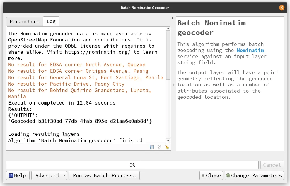
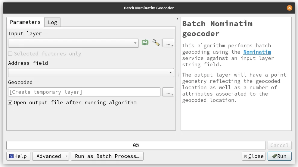
Geocoding algorithms

QGIS has a native geocoding processing algorithm called Batch Nominatim geocoder and geocoding capabilities using the MMQGIS plugin. Both these tools require a table or layer with at least one field containing address information, such as street address, city, state, and zip code. In the case of the former only street address is required.

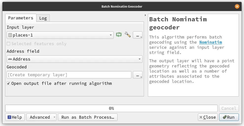
To geocode addresses using the Batch Nominatim geocoder processing algorithm:

1. Make sure the Processing plugin is activated.
2. Search for the Batch Nominatim geocoder algorithm and run it to open the processing window.
3. In the processing window window, provide the parameters for the input layer and address field then run the algorithm.

Figure 6. The Batch Nominatim Geocoder

To geocode addresses using the “MMQGIS Geocode” plugin:

1. Make sure the plugin is installed and activated. You should find an MMQGIS menu added to the Menu bar.
2. Click on the MMQGIS menu and select Geocode from the dropdown. There are three options for geocoding:
   1. Geocode CSV with Web Service
   2. Geocode from Street Layer
   3. Reverse geocode

Figure 7. Web Service Geocode using the MMQGIS plugin

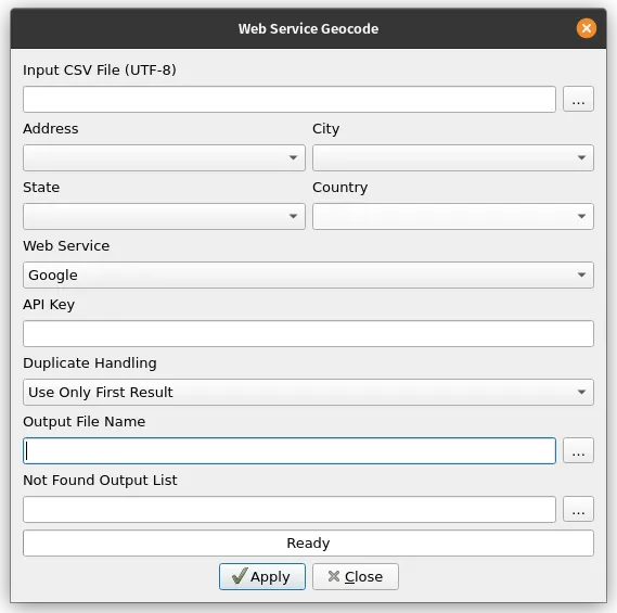
3. In the Geocode CSV with Web Service, you can provide information such as the input CSV, fields for the address, city, country, and even what web service to use for geocoding.

NOTE

Some geocoding web services require an API key.

PRO-TIP

Nominatim is a free and open-source geocoding based on OpenStreetMap data that converts addresses into geographic coordinates (latitude and longitude) and vice versa. Being based on OSM, the quality and completeness of the location information may vary depending on the availability and accuracy of the OpenStreetMap data in the area. It is always a good practice to cross-check the results with other data sources and to manually adjust the geocoded locations if necessary.

Additionally, it is recommended to use Nominatim with moderation and respect for the OpenStreetMap community’s resources and guidelines, as excessive or abusive use can result in temporary or permanent suspension of the geocoding service.

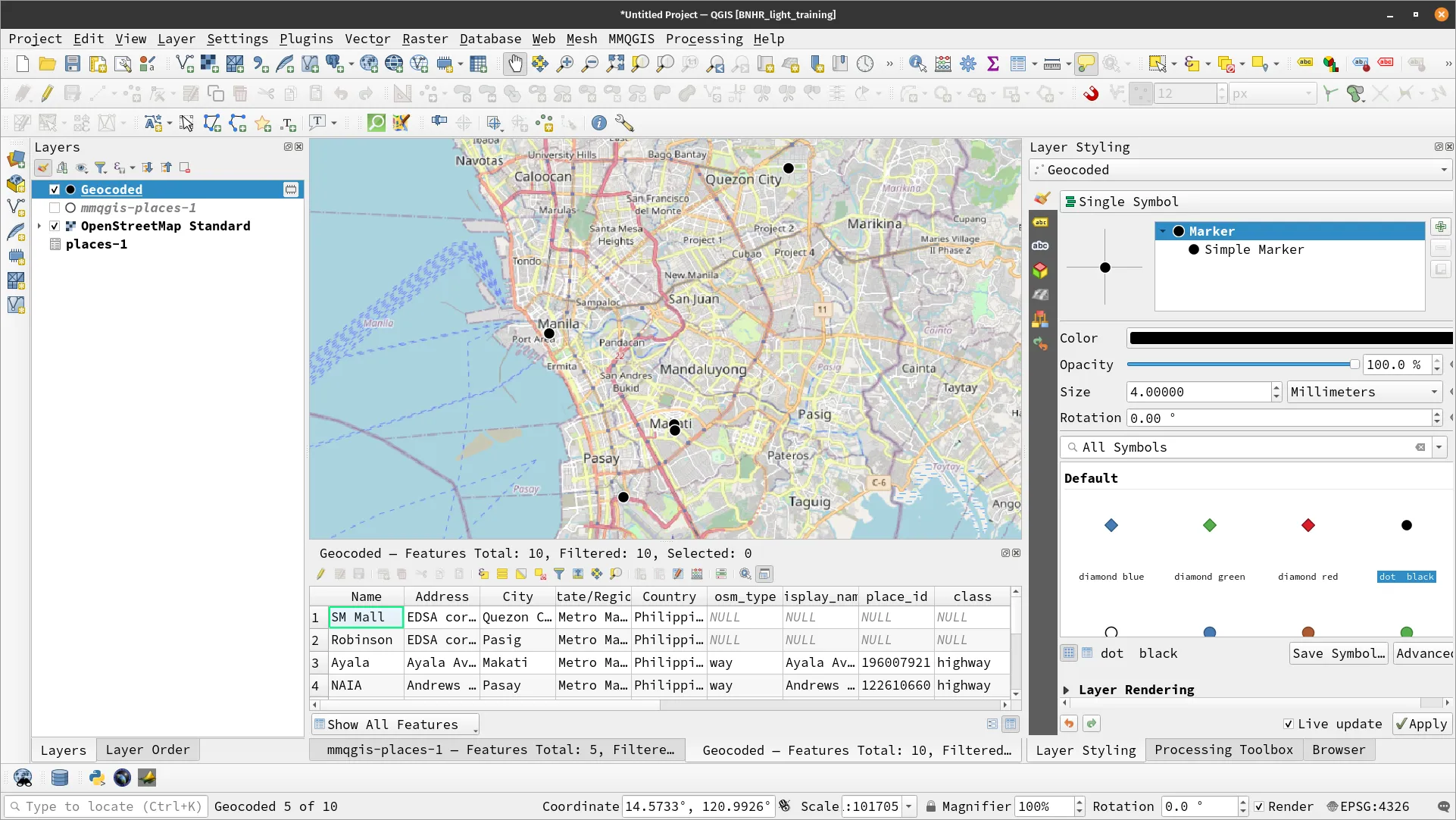
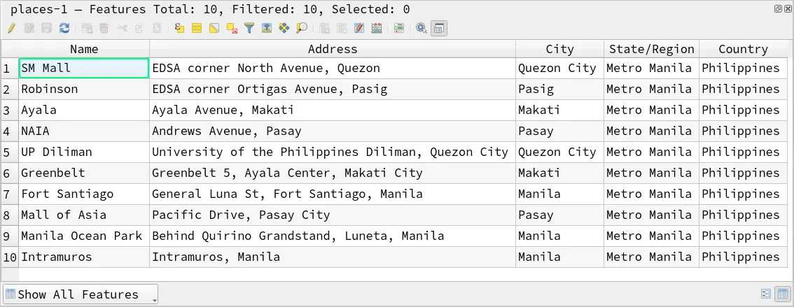
Exercise 3.2. Geocoding a set of addresses

You will use the places-1.csv and places-2.csv found in the data folder.

1. Open places-1.csv to see its fields and values. You can use your preferred text editor, spreadsheet application, or you can load the CSV in QGIS as a layer. You will use the Address, City, State/Region, and Country fields to geocode the layer.

Figure 8. The places-1.csv. Notice the values for the address, city, etc.

2. First, try it with the MMQGIS plugin.
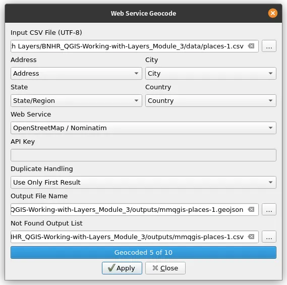
3. Open the Geocode CSV with Web Service tool and input the following parameters:

Figure 9. Geocoding places-1 with MMQGIS

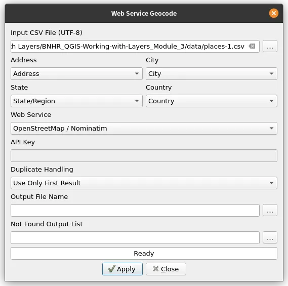
4. Don’t forget to select the Output File and Not Found Output List.
   1. The Output File will be a vector layer containing the points that were successfully geocoded—this can be in any vector layer format such as geopackage or shapefile.
   2. The Not Found Output List
5. Click Apply.
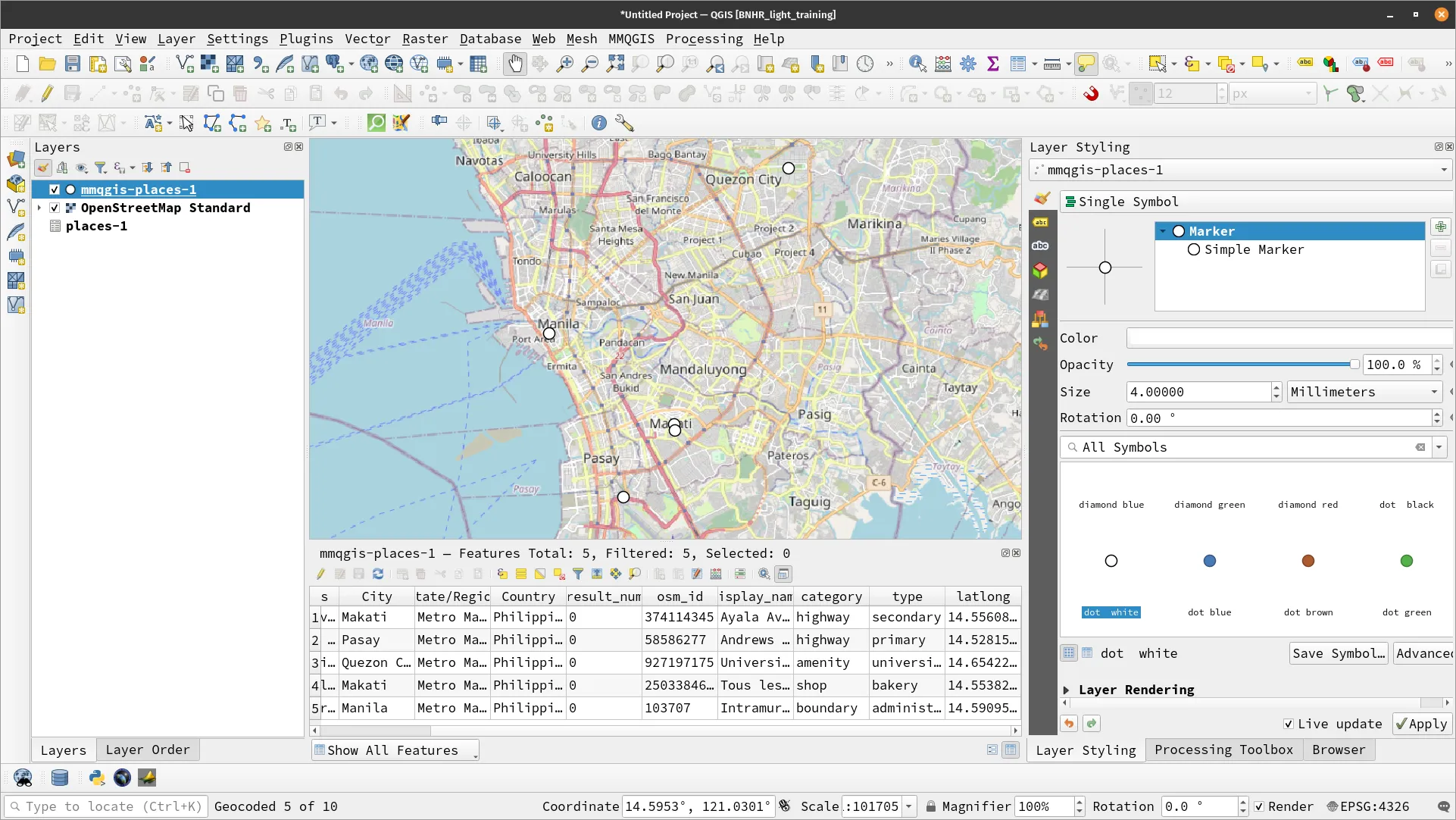
6. Did all the places get geocoded? Are the geocoded places correct?

Figure 10. places-1 geocoded with MMQGIS

Figure 11. Results of places-1 geocoding with MMQGIS

7. Now try to do the same with the Batch Nominatim geocoder algorithm.
8. Open the algorithm and input the following parameters:

Figure 12. arameters for geocoding places-1 with the Batch Nominatim geocoder

9. Did you get the same results as the MMQGIS plugin?

Figure 13. Batch Nominatim geocoder results

Figure 14. Results of places-1 geocoding with Batch Nominatim geocoder

10. Now try to geocode places-2.csv.

SOMETHING TO THINK ABOUT

What do you think are the advantages and disadvantages of using the Batch Nominatim geocoder and the MMQGIS plugin?

Memory boosters and review

What is geocoding?

The process of converting location data such as addresses, place names, or postal codes into geographic coordinates.

What are the factors that can affect geocoding accuracy?

Data quality, consistency, and completeness of the input data, as well as the accuracy and quality of the reference data used for geocoding.

How can you check the accuracy of your geocoded data?

By visualizing the geocoded points on a map and comparing them with other known locations or spatial data.

What geocoding tools are available in QGIS?

Native processing algorithms such as Batch Nominatim geocoder or plugins such as MMQGIS

What are the input requirements for geocoding in QGIS?

To geocode addresses in QGIS, you need a table or layer with at least one field containing address information, such as street address, city, state, or country.

What to do when: you have a digital image or map of an area but it doesn’t load in the correct location

LEARNING OBJECTIVES

1. Understand what georeferencing is and why it is important
2. Learn how to georeference a layer in QGIS
3. Understand how to check the accuracy of a georeferenced layer

Georeferencing

Georeferencing is the process of assigning geographic information to a layer in order to place it on its proper world location. This is done:

• by selecting common features between the layer and another georeferenced layer or
• by inputting the coordinates of the pixels directly.

The latter method is used when the pixel coordinates are known, such as in a map with a grid showing the coordinates of the grid. The former method involves using a second image with known geographic information, typically by identifying easily recognizable features in both images.

NOTE

Learn more about georeferencing in the QGIS User Manual.

• Raster Georeferencing

Why do we georeference?

Georeferencing is an important feature of any GIS because it allows you to se non-georeferenced data sources such as old maps, hard-copy maps, hard-copy aerial imagery, photographs, and more. By georeferencing non-georeferenced data, we can unlock valuable historical, cultural, or environmental information that would otherwise be inaccessible for spatial analysis.

How do we georeference?

Georeferencing works because of a process known as coordinate transformation.

Recall: We discussed in the Essentials that a coordinate reference system is a set of points that is used to define the position of an object on the surface of the earth. Different coordinate reference systems have different parameters or functions that define their set of coordinates and you can compute for transformation parameters between two coordinate reference systems.

If we have two layers showing the same location but in different coordinate reference systems, we can compute for the transformation parameters between the two coordinate reference systems as long as we have enough points in both layers that we know the coordinates of (commonly referred to as Ground Control Points or GCPs).

You can select different transformation types to aid you in georeferencing, these include (in order of increasing computational complexity):

• Linear transformation – preserves parallelism and straight lines. It is one of the simplest transformation types as it only involves rotation, scaling, and translation. Mathematically, it can be represented by a matrix of numbers multipled by a vector of coordinates.
• Helmert transformation – is a type of Affine transformation that involves rotation, scaling, translation, and a shift (shear or skew) component.
• Projective transformation – is used when the image has a perspective distortion or non-linear distortions.
• Other higher order transformations
  • Polynomial transformation – involves fitting a polynomial function to a set of control points to determine the transformation parameters. The polynomial function can be of various orders, such as first-order, second-order, third-order, etc., depending on the level of distortion in the image.
  • Thin plate spline transformation – involves creating a smooth surface that passes through a set of control points and uses this surface to transform the image.

PRO-TIP

Do not think that you should always go for the most complex transformation type. The choice should always depend on the actual context of the layer being georeferenced.

When selecting the transformation parameters, you must consider:

• the layer’s complexity and distortion (regular-shaped maps normally only need to use simple transformation parameters)
• the number of GCPs that you can get on the map—the more complex the transformation type, the more GCPs are needed to get good results
• the distribution of GCPs on the map—poor GCP distribution results in more distortion especially in higher order transformation equations
• more (or more complex) is not always better

The table below shows the recommended minimum number of GCPs required depending on the order of transformation that you will use:

Order of Transformation	Minimum GCPs Required
1	3
2	6
3	10
4	15
5	21
6	28
7	36

Just to be safe, always have at least one more than the minimum to add redundancy to the transformation computations.

Raster and vector georeferencing

NOTE

QGIS 3.26 introduced vector georeferencing. Prior to this version, only rasters could be georeferenced in QGIS but starting version 3.26, vectors could also be georeferenced. This also moved the Georeferencing command from the Raster menu to the Layer menu.

The usual workflow for georeferencing a layer in QGIS is as follows:

1. Open the Georeferencer window (accessible from Layer ‣ Georeferencer… in QGIS 3.26 and newer, Raster ‣ Georeferencer… for older versions)
2. Add/open the layer to be georeferenced.
3. Define the transformation settings
4. Add the ground control points by zooming in the area of interest, clicking a point, and:
   1. adding the coordinates; or
   2. selecting the corresponding point on the map canvas.
5. Perform the coordinate transformation by clicking Start georeferencing.
6. Check the results in the Map Canvas

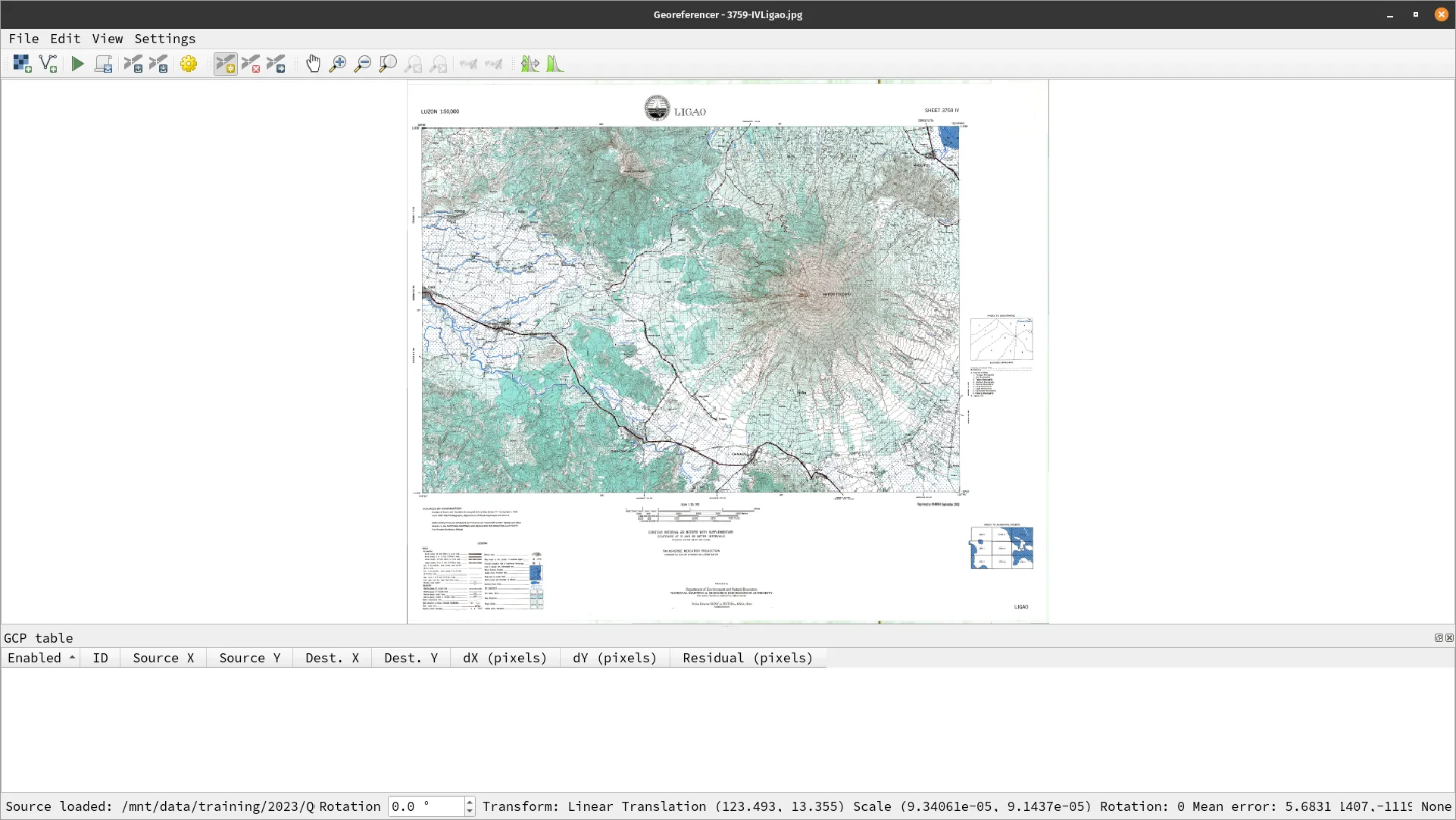
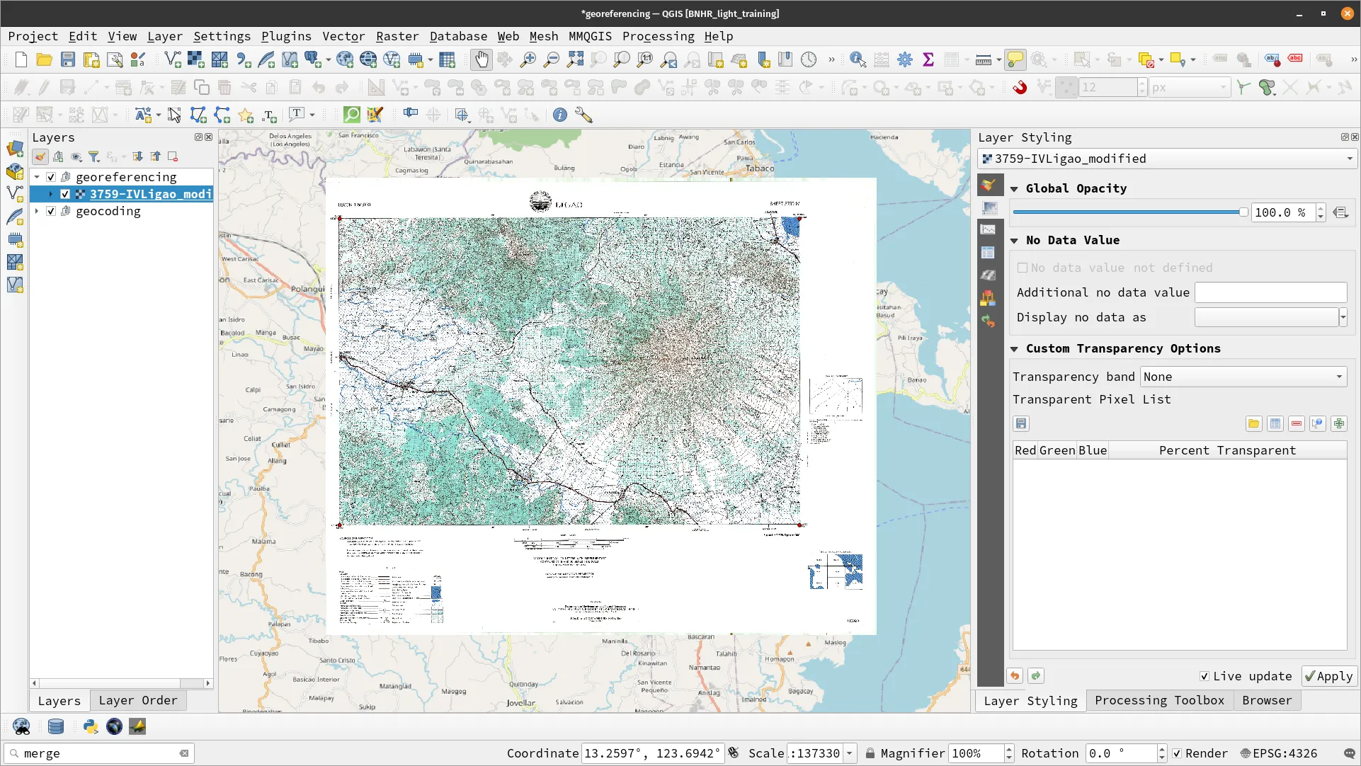
The Georeferencer window

Figure 15. The Georeferencer window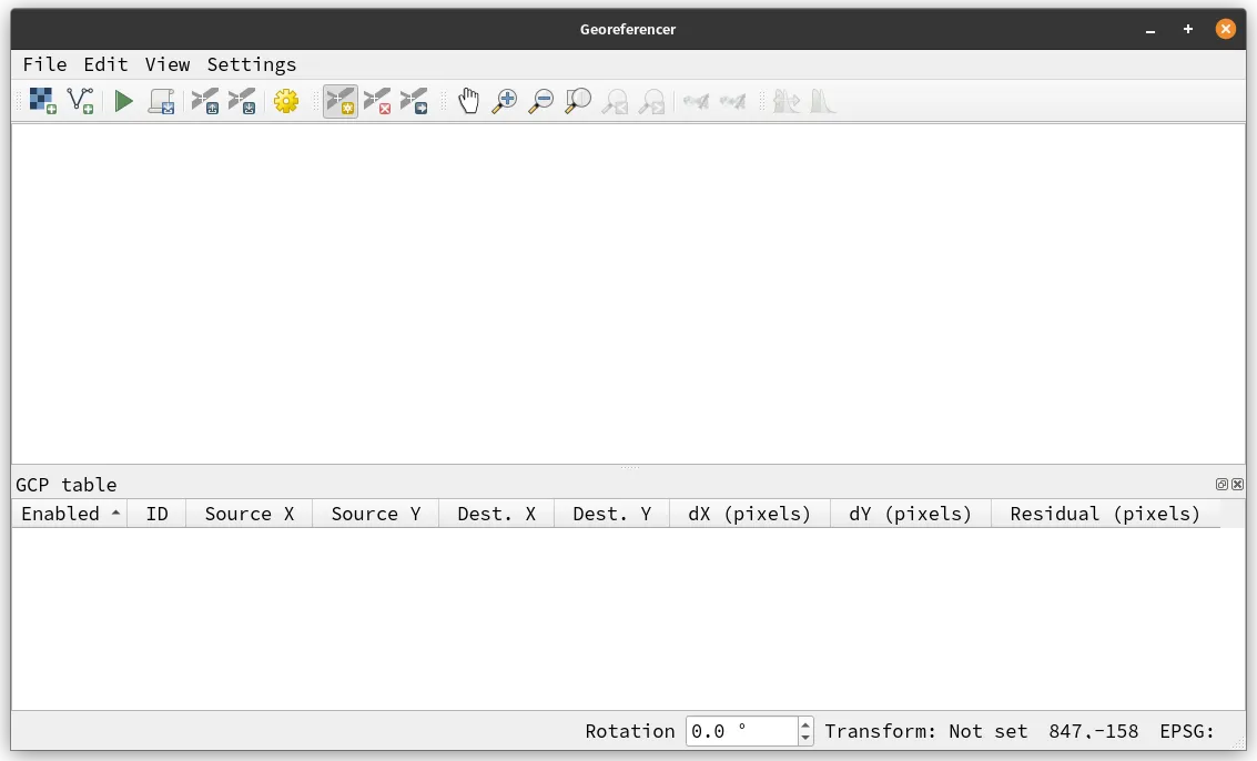 in QGIS

The Georeferencer window looks similar to the main QGIS window. It has a Menu bar, toolbars, panels, as well as a georeferencer canvas in the middle. The Georeferencer window has four menus: File, Edit, View, and Settings. Generally speaking:

• The File menu allows users to open files to be georeferenced, load or save Ground Control Points (GCPs), and generate a GDAL script.
• The Edit menu provides options for adding, removing, or editing GCPs.
• The View menu contains options for zooming in or out, panning the image or map, and viewing the entire georeferenced layer. It also controls linking the georeferencer canvas with the main QGIS map canvas as well as the visibility of toolbars and panels.
• The Setting menu allows you to configure the georeferencer ant the transformation settings.

Figure 16. Georeferencer menu bar

Each menu also has a corresponding toolbar.

Figure 17. File toolbar

Figure 18. Edit toolbar

Figure 19. View toolbar

The main canvas in the Georeferencer window is where you will perform your georeferencing. It displays the layer that you load for georeferencing, and it is where you will select your Ground Control Points (GCPs). The canvas also provides visual feedback on the current errors and distortions of the georeferenced layer.

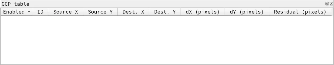
Additionally, the Georeferencer window includes a GCP Table panel that displays a list of all the GCPs you’ve added to the layer. This panel allows you to edit the GCPs’ coordinates or delete them. It also shows the error and residual values for each GCP giving you detailed information on the accuracy of your georeferencing.

Figure 20. GCP table panel

Exercise 3.3. Georeferencing a raster in QGIS

You will use the 3759-IVLigao.jpg image inside the data folder

1. Open the Georeferencer.
2. Open the 3759-IVLigao.jpg image using File ‣ Open Raster (CTRL + O) in the Menu bar or from the File toolbar.

Figure 21. Ligao topo map loaded in the Georeferencer

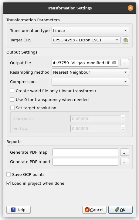
3. Next, set the transformation settings for georeferencing this layer. Go to Setting ‣ Transformation Settings or click the Settings button () from the File toolbar. Use the following parameters:
   • Transformation type: Linear
   • Target CRS: EPSG: 4253 – Luzon 1911
   • Output file: as preferred
   • Resampling method: Nearest Neighbor

SOMETHING TO THINK ABOUT

Why did you use EPSG: 4253 – Luzon 1911 as the target CRS?

Figure 22. Transformation settings

4. Start adding Ground Control Points by enabling Edit ‣ Add point (CTRL + A) or clicking the Add GCP Point () from the Edit toolbar. Your cursor should become a crosshair.

Figure 23. Crosshair for adding GCP

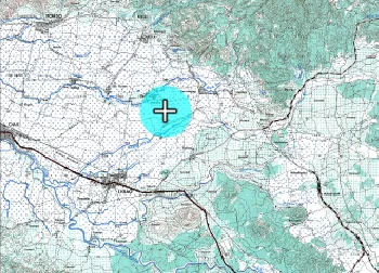
5. Thankfully, the map already gives us the coordinates of certain points. Because of this, we can simply select these points and add their corresponding coordinates.

SOMETHING TO THINK ABOUT

If we didn’t have coordinates on the map, what would we do to georeference the image?

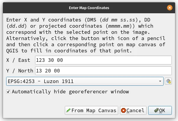
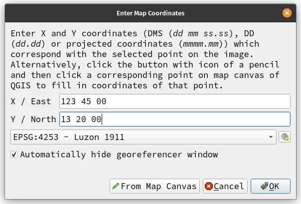
6. Zoom to one of the corners of the map. Notice that it has a coordinate values. Click on the corner with your cursor. Be as precise as possible.

Figure 24. Adding a GCP

7. This should open the Enter Map Coordinates dialog. Input the coordinates here. Make sure to follow the proper format (dd mm ss.ss, dd.dd, or mmmm.mm).

Figure 25. Adding the coordinates

8. Repeat this process 3 more times for a total of 4 GCPs.

NOTE

Remember that a 1st order transformation or a Linear transformation requires at least 3 GCPs.

Figure 26. Adding more GCPs

Figure 27. Adding more coordinates

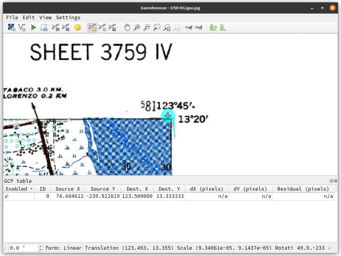
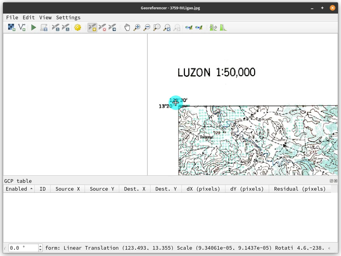
9. After adding enough GCPs, your canvas should look like:

Figure 28. Ready for georeferencing

10. Take note of the red lines on the canvas and the GCP table as these provide you information on the accuracy of your georeferencing.

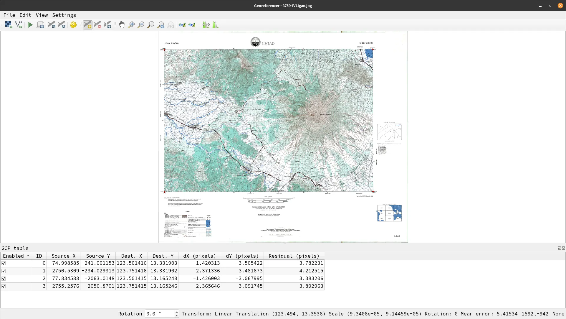
11. Once you’re satisfied with the GCPs and residuals, start the georeferencing by going to File ‣ Start Georeferencing or clicking the Start Georeferencing button () on the File toolbar.

12. A new layer should appear on your map canvas.

13. Perform some visual quality checks on the results of your georeferencing.

Figure 29. Georerefenced Ligao topo map

PRO-TIP

If we didn’t have coordinates on the map, we would use the button to find corresponding points on both the the Ligao topo map and the map canvas in QGIS. This requires us to have an already georeferenced map in our map canvas—e.g. satellite imagery, basemaps, etc.—and to find features that are easily identifiable on both maps.

Memory boosters and review

What is georeferencing?

Georeferencing is the process of aligning a digital image or map to real-world coordinates.

Why is georeferencing important in GIS?

It enables you to properly locate your data, overlay it on top of other layers, and perform spatial analysis.

What are some techniques for improving the accuracy of georeferenced layers?

Adding more control points or using more complex transformation are techniques for improving the accuracy of georeferenced layers.

What are ground control points?

In the context of georeferencing, ground control points refer to points whose real world coordinates are known or those whose coordinates are known in both the source layer and in the target layer to be georeferenced.

How can you deal with distorted or warped images in georeferencing?

You can use advanced techniques such as polynomial transformation to deal with distorted or warped images in georeferencing.

What to do when: you need to create a new layer

LEARNING OBJECTIVES

1. Understand how to create a new vector layer in QGIS.
2. Learn about the concept of virtual vectors and virtual rasters.

Creating a new layer in QGIS is an essential task for any GIS project. In this chapter, we’ll explore how to create a new vector layer, as well as the concept of virtual vectors and virtual rasters, which can be useful in certain situations.

Creating a new vector layer

There are several ways to create a new vector layer in QGIS and several vector formats that can be created. You can find most of them under Layer ‣ Create Layer or via the Data Source Manager toolbar.

Figure 30. Data Source Manager toolbar

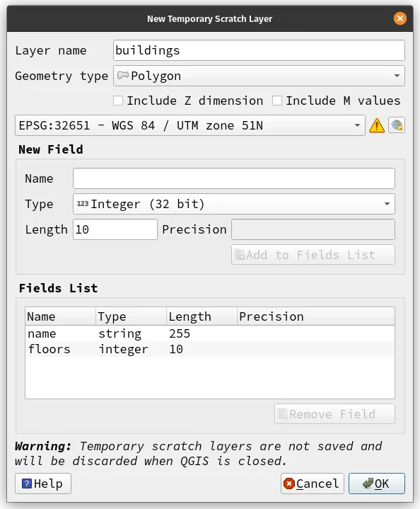
No matter what type of vector layer you create, the initializaton process follows similar steps:

1. You need to provide:
   1. the name of the layer,
   2. the geometry you want to use for the layer—e.g. point, line, polygon, etc.,
   3. the Coordinate Reference System for the layer,
   4. the fields of the layer.

Figure 31. Creating a new buildings polygon layer in WGS84 with several fields

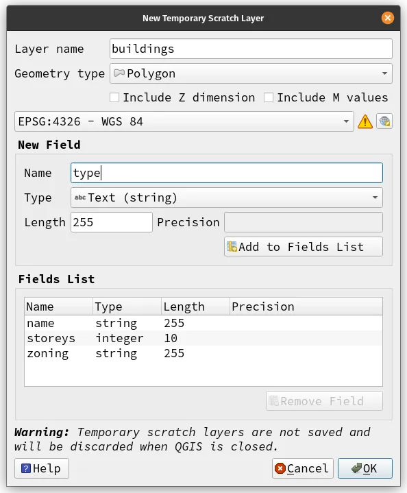
After creating the layer, it should appear on your Layers panel.

Virtual vectors and virtual rasters

In some situations, you may not want to create a new layer in your project, but you still need to access and work with the data. This is where virtual vectors and virtual rasters can be useful.

QGIS has built-in processing algorithms for creating virtual vectors and rasters: Build virtual vector and Build virtual raster.

Virtual vectors and virtual rasters are a way to combine several layers and treat them as if they were a single vector or raster layer within QGIS.

NOTE

Similar to Virtual layers, Build virtual vector appears to not work for Temporary layers or layers in memory.

What to do when: you have an image or map and you need to extract information from it

LEARNING OBJECTIVES

1. Understand the concept of digitizing
2. Know how to digitize features in QGIS

By georeferencing, we are able to put maps in their proper location on the earth. However, sometimes this is not enough and what we need is to extract data from the maps that we can use as vector layers. This is where the process of digitizing comes in.

In the context of QGIS, digitizing refers to the process of converting analog maps, satellite imagery or other types of paper-based or non-digital data into digital format by manually tracing features using a mouse or other pointing device. Digitizing is an essential tool for creating new maps, updating old maps or adding new features to existing maps.

NOTE

To start digitizing data, Editing mode must be toggled on for the vector layer.

PRO-TIP

To start digitizing data, Editing mode must be toggled on for the vector layer.

PRO-TIP

You can restrict edit permissions of layers in a project by setting them as read-only from the Project ‣ Properties ‣ Data Sources ‣ Layers Capabilities table. This works regardless of the provider permission.

Enabling this feature can be a useful method in a multi-user environment to prevent unauthorized users from unintentionally modifying layers and potentially damaging the data. However, it’s important to note that this configuration only applies within the current project.

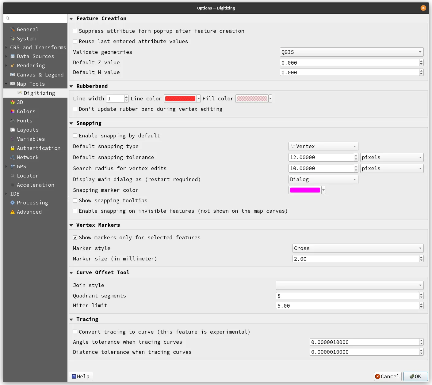
Digitizing Settings

Digitizing settings can be found under Settings ‣ Options ‣ Digitizing tab. Here, you can set options for feature creation, snapping, and other useful parameters when digitizing data.

Figure 32. Digitizing settings

About snapping

Digitizing layers in QGIS involves creating and editing vector layer geometries. One important aspect of digitizing is setting an appropriate value of snapping tolerance and search radius for feature vertices. QGIS provides a number of parameters to configure the default behavior of editing tools.

The snapping tolerance is the distance QGIS uses to search for the closest vertex or segment when adding a new vertex or moving an existing one. If the vertex is not within the snapping tolerance, QGIS will leave the vertex where you release the mouse button, instead of snapping it to an existing vertex or segment. The search radius is the distance QGIS uses to search for the vertex to select when you click on the map. If the vertex is not within the search radius, QGIS will not find and select any vertex for editing.

You can set the snap tolerance and search radius in the Settings ‣ Options ‣ Digitizing menu. Snapping and digitizing settings (snapping mode, tolerance value, and units) can also be overridden in the project from the Project ‣ Snapping Options menu. You can also use the Snapping toolbar.

There are three options to select the layer(s) to snap to: all layers, current layer, and advanced configuration. All layers is a quick setting for all visible layers in the project, while current layer only uses the active layer. Advanced configuration allows you to enable and adjust snapping mode, tolerance, and units, overlaps, and scales of snapping on a layer basis.

By default, only visible features can be snapped. You can enable snapping on invisible features by checking Enable snapping on invisible features under the Settings.

Snapping mode allows you to choose between Vertex, Segment, Area, Centroid, Middle of Segments, and Line Endpoints. The tolerance values can be set either in the project’s map units or in pixels.

Another available option is to use snapping on intersection, which allows you to snap to geometry intersections of snapping enabled layers, even if there are no vertices at the intersections.

Snapping can become very slow if there are a lot of features in some layers that require a heavy index to compute and maintain. You can limit snapping to a scale range to avoid this issue. Limiting snapping to a scale range is only available in Advanced Configuration mode and can be configured in Project ‣ Snapping Options.

NOTE

For more information, you can refer to the QGIS User Manual.

Digitizing toolbar

The Digitizing toolbar contains basic commands that will allow you to digitize data.

NOTE

For more information, you can refer to the QGIS User Manual.

Advanced digitizing toolbar

The advanced digitizing toolbar has functions for:

• moving, rotating, and scaling features
• copying, moving, and reshaping features
• splitting and merging features
• adding, filling, and deleting rings
• adding, deleting, and splitting parts
• and many more

NOTE

For more information, you can refer to the QGIS User Manual.

Shape digitizing toolbar

The Shape Digitizing toolbar offers a set of tools to draw regular shapes and curved geometries.

This includes:

• Adding circular strings
• Drawing circles
• Drawing ellipses
• Drawing rectangles
• Drawing regular polygons

NOTE

NOTE: For more information, you can refer to the QGIS User Manual.

Advanced digitizing panel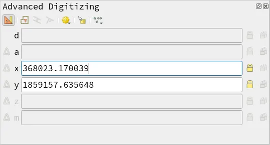

The Advanced Digitizing panel is a tool in QGIS that provides advanced functionality for capturing, reshaping, splitting new or existing geometries with greater precision and accuracy. The panel can be from the View ‣ Panels menu or pressing Ctrl+4.

Once the panel is visible, you can activate the advanced digitizing tools by clicking the Enable digitizing tools buttton () from the Advanced Digitizing toolbar. However, it is important to note that these tools are not available if the map view is in geographic coordinates.

NOTE

CAD tools are not enabled if the map view/canvas is in geographic coodinates.

The aim of the Advanced Digitizing tool is to allow users to lock coordinates, lengths, and angles when moving the mouse during the digitizing process in the map canvas. This means that users can draw lines that are exactly parallel or perpendicular to a particular angle or lock lines to specific angles. Furthermore, users can enter coordinates directly, making it possible to define new geometries with greater accuracy.

In addition to locking coordinates, lengths, and angles, the Advanced Digitizing panel allows users to create constraints with relative or absolute reference. Relative reference means that the next vertex constraint values will be relative to the previous vertex or segment. This makes it easier to create complex geometries that require precise measurements and angles.

NOTE

For more information, you can refer to the QGIS User Manual.

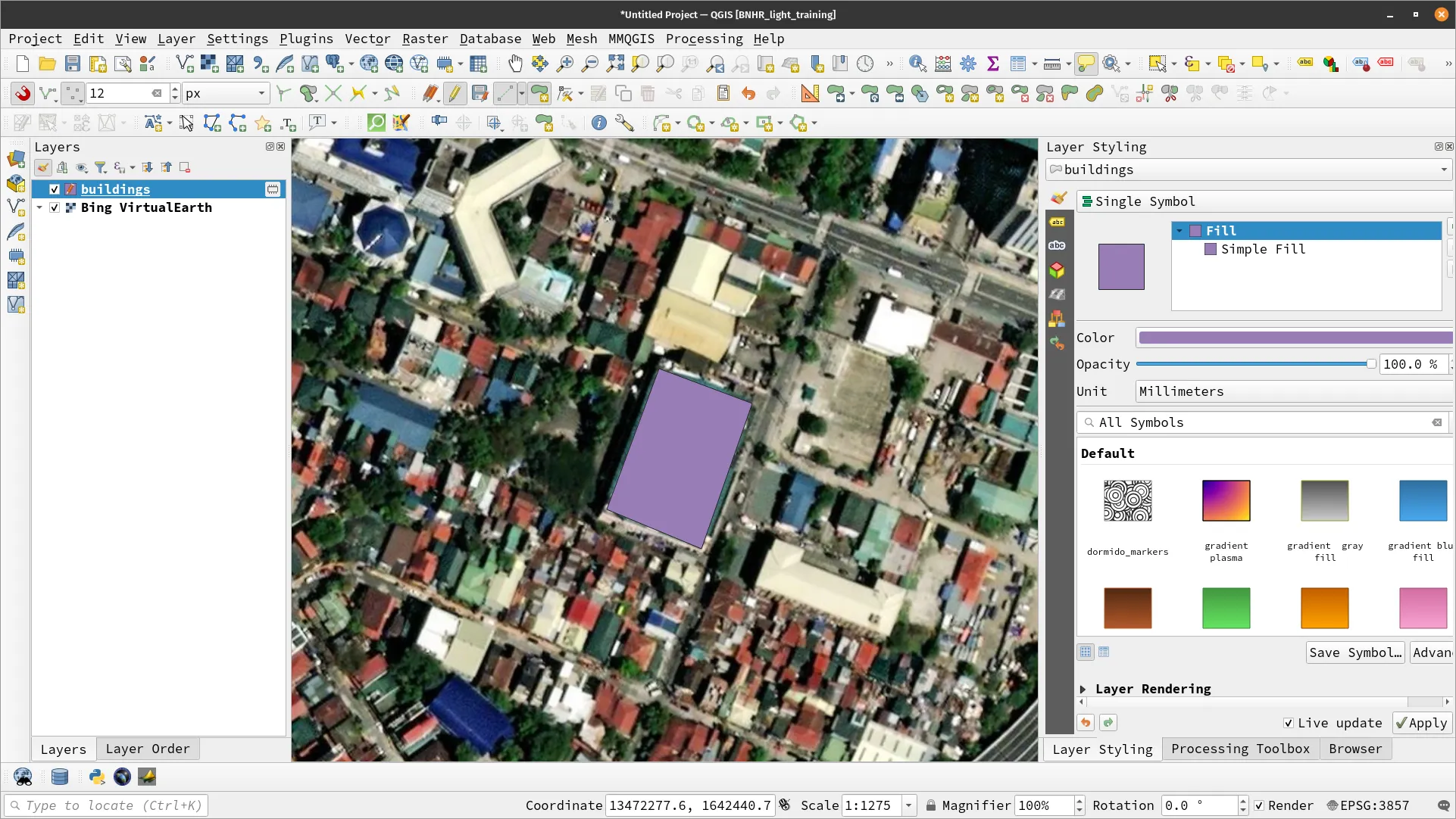
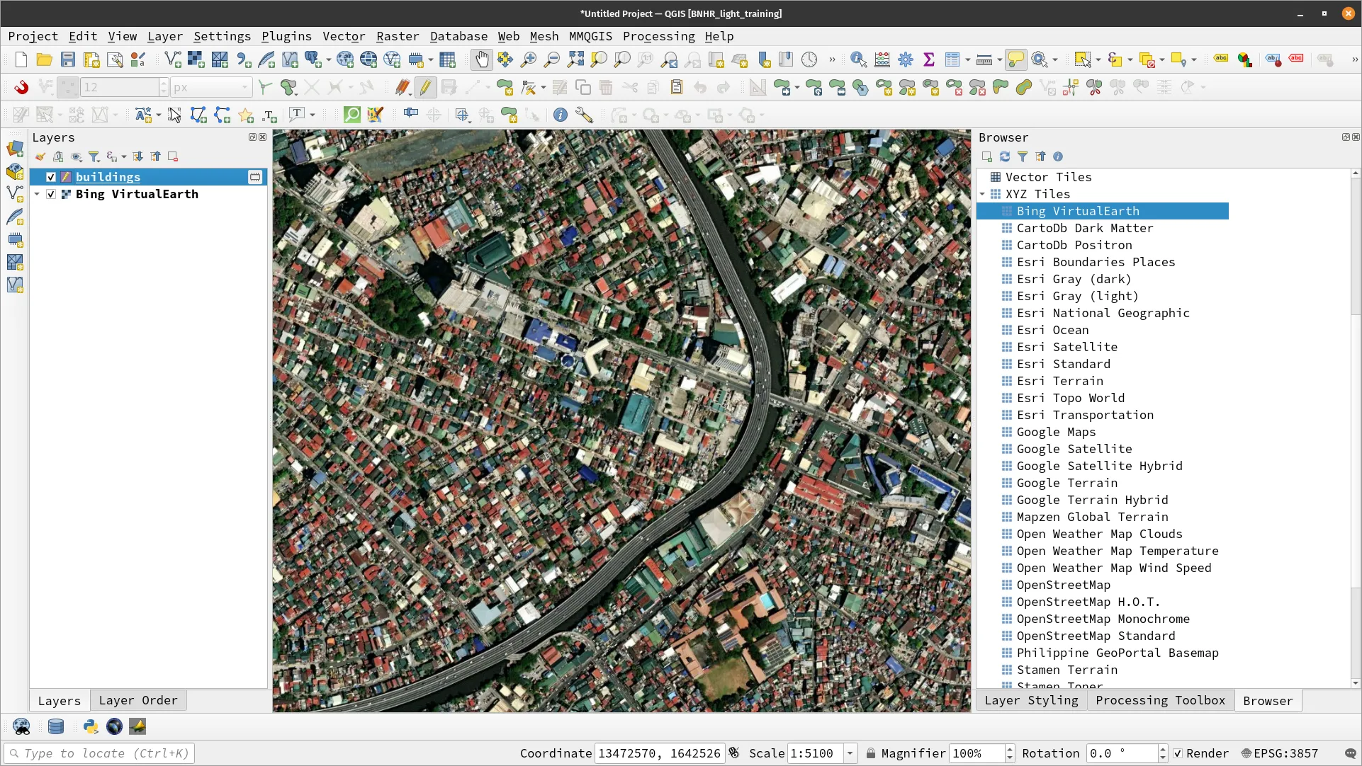
Exercise 3.4. Digitizing new buildings

In this exercise, we will try to digitize buildings on a map.

1. Load a satellite image basemap like Bing VirtualEarth.
2. Create a new vector layer for your buildings.

Figure 33. New vector layer for buildings

3. Select buildings in the Layers panel and makes sure to enable editing on the layer (right-click ‣ Toggle Editing).

4. Click on the Add Feature (CTRL + .) button () to start digitizing.

Figure 34. Editing mode on buildings

5. To begin, click on one of the building’s corners and then continue placing additional points by clicking on the remaining corners or tracing the building’s outline until the entire structure is enclosed. Essentially, this process is akin to drawing a polygon.

Figure 35. Digitizing a building

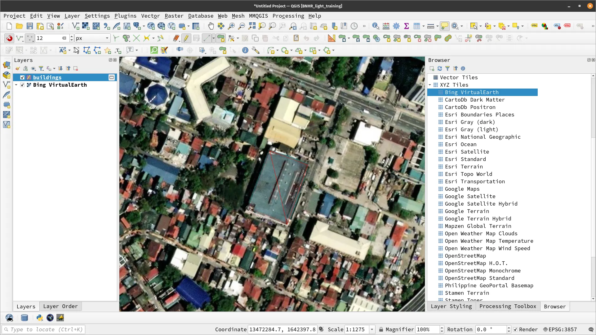
6. Right-click to complete digitizing a feature. This will open the feature attribute form that will ask you to provide values for the feature attributes/fields.

Figure 36. Add attributes to the digitized feature

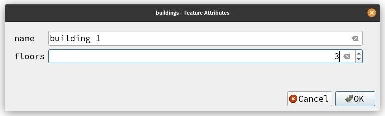
7. Your digitized feature should now appear on the map.

Figure 37. Digitized feature on the map

8. Add more building features to the layer and don’t forget to save your edits!

Memory boosters and review

What is digitizing?

The process of “tracing” or “extracting” information from media/maps to create new vector data.

What should you use if you want to be able to create shapes and polygons when digitizing?

Shape digitizing toolbar

What should you use if you want to be have CAD-like capabilities when digitizing?

Advanced digitizing panel

How do you start digitizing in QGIS?

To start digitizing in QGIS, open the layer you want to edit, toggle editing mode, and then use the digitizing tools to add or edit features.

How can you ensure accuracy while digitizing in QGIS?

To ensure accuracy while digitizing in QGIS, you can use various tools, such as the Snapping options, to align new features with existing ones, and the Vertex Editor to adjust the position of individual vertices.

BONUS: Mapping tracts acts of land from technical descriptions and land titles

LEARNING OBJECTIVES

Learn how to use QGIS for mapping tracts or parcels of land from technical descriptions or land titles

In mapping tracts of land from technical descriptions and land titles, the most difficult part is getting the coordinates of the tie-point. Once this is known, it becomes as simple as using a plugin.

Azimuth and Distance Plugin

The Azimuth and Distance Plugin is one of the simplest means to map survey returns (e.g. bearings and distances). It can be installed from the Manage and Install Plugins dialog.

Figure 38. Azimuth and Distance Plugin

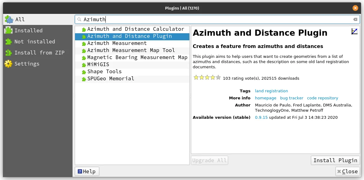
Inputs to the plugin can be done manually in QGIS or through an input file (which is basically a text file that tells the plugin about what data to plot).

Figure 39. Azimuth and distance plugin interface

Exercise 3.5. Mapping land parcels with the Azimuth and Distance plugin

1. Set the options in the Options tab.
   • Survey type: Boundary
   • Angle type: Bearing
   • Distance unit: Default
   • Angle unit: Degree

Figure 40. Sample options for the Azimuth and Distance plugin

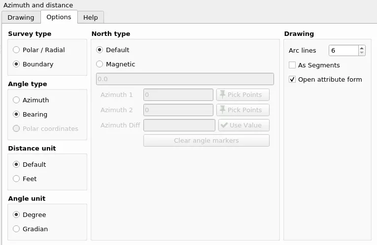
2. Set the CRS of the project to the correct CRS. Projected CRS (e.g. PRS92 Projected 51N, UTM Zone 51N, etc.) are usually preferred.

SOMETHING TO THINK ABOUT

Why do we use projected CRS in mapping land parcels?

3. Create or select a layer to hold the data to be mapped (optional). If a layer is not created, the data will be stored as a layer in memory.
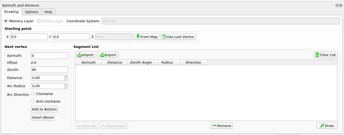
4. Go to the Drawing tab.
5. Add the coordinates of the Starting Point. You can also select this from the map if needed.
6. Add the bearing and distance parameters. a. Azimuth: Bearing in N/S DD MM SS.SS E/W b. Distance: Distance
7. Click Add to Bottom or Insert Above depending on where the observation should be.
8. Repeat until all observations or bearings and distances have been added.
9. When adding a new observation, the line is automatically shown as a preview.
10. To draw the line or create a vector layer in QGIS, click the Draw button ()

Figure 41. Sample usage of the Azimuth and Distance plugin

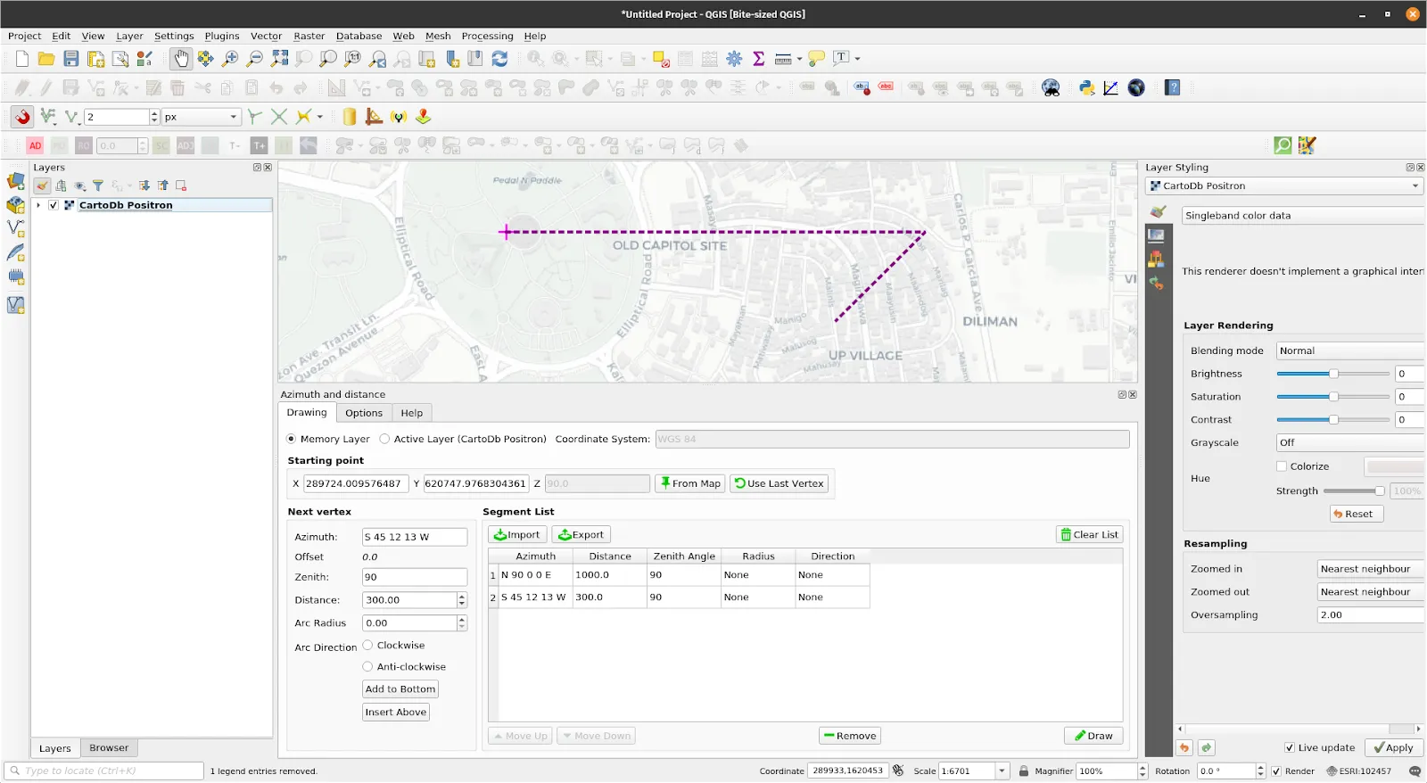
11. You can also import and export parameters via the Import and Export buttons.

Tip to make it easier

There is a more efficient method to prepare input data for the Azimuth and Distance plugin in QGIS. Instead of manually entering values, you can create a text file beforehand using any text editor. The file format is simple, with the first few lines containing information on the survey’s starting point and values provided in the Options tab. The remaining lines under the [data] section correspond to the bearings, distances, zenith, angle, and direction of each observation.

angle=Bearing
heading=Coordinate_System
dist_units=meters
angle_unit=degree
startAt=289724.009576487;1620747.9768304361;90
survey=Polygonal
[data]
N 90 0 0 E;1000.0;90;None;None
S 45 12 13 W;300.0;90;None;None

PRO-TIP

The import file of the plugin is simply a text file which can be opened with any text editor.

You can easily modify the text file to include all observations for a survey, making the importing process faster and more convenient. The edited file can then be imported into the plugin with ease.

Certification and support

LOOKING FOR CERTIFICATION AND SUPPORT?

We offer additional resources, certificates, official QGIS certification, ongoing support, and other perks to those who avail of our paid courses.

Contact us or sign-up to our courses if you are interested in having this as an instructor-led or self-paced course.