Advanced Styling Techniques

Introduction

This module will teach you advanced styling techniques such as blending modes, geometry generators, data-defined overrides, and draw effects.

What you should already know

As an intermediate level course, you are expected to already know basic GIS concepts such as spatial data models and formats and QGIS functions such as loading and styling layers, running processing algorithms, saving QGIS projects, etc.

LEARNING OBJECTIVES

1. Learn how to use advanced styling techniques in QGIS such as:
   • Blending modes
   • Geometry generators
   • Data-defined overrides
   • Draw effects

NOTE

For exercises 2.X in this course, you will use the bnhr_qgis-advanced-styling.gpkg inside the data subfolder in the BNHR_QGIS-Advanced-Styling-and-Symbology folder.

This geopackage contains all the data and projects associated with the exercises.

Blending modes

Similar to graphics manipulation applications such as GIMP and Photoshop, QGIS has what’s called Blending Modes that allow for more sophisticated rendering between GIS layers. These blending modes refer to the techniques used to combine different map layers visually that enhance their overall appearance and readability. They determine how the colors of one layer interact with the colors of underlying layers which—when done well—allows you to achieve specific visual effects.

There are 13 blending modes which (aside from the Normal mode) can be divided into four groups. These modes are:

• Normal
• Lighten
  • Lighten
  • Screen
  • Dodge
  • Addition
• Darken
  • Darken
  • Multiply
  • Burn
• Contrast
  • Overlay
  • Soft light
  • Hard light
• Inversion/Cancellation
  • Difference
  • Subtract

Technically speaking, some of these blending modes refer to the following processes:

• Normal: This is the standard blend mode, which uses the alpha channel of the top pixel to blend with the pixel beneath it. The colors aren’t mixed.
• Lighten: This selects the maximum of each component from the foreground and background pixels. Be aware that the results tend to be jagged and harsh.
• Darken: Retains the lowest values of each component of the foreground and background pixels. Like lighten, the results tend to be jagged and harsh.
• Difference: Subtracts the top pixel from the bottom pixel, or the other way around, in order always to get a positive value. Blending with black produces no change, as the difference with all colors is zero.

NOTE

Learn more about the other blending modes at https://docs.qgis.org/latest/en/docs/user_manual/introduction/general_tools.html#blending-modes

Figure 1. Examples of blending modes applied to a green feature over an orange feature (from the QGIS user manual)

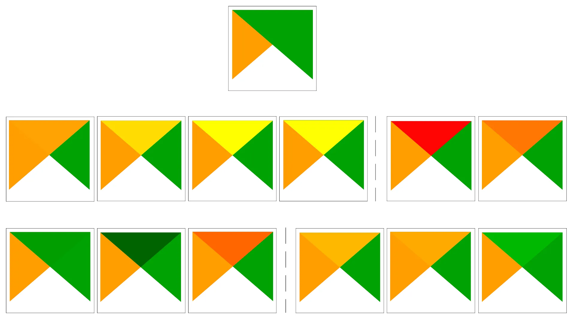
• Top row: Normal
• Middle row (left to right): Lighten, Screen, Dodge, Addition, Difference, Subtract
• Bottom row (left to right): Darken, Multiply, Burn, Overlay, Soft light, Hard light

Aside from blending individual layers, when a layer is part of a group, additional blending modes for rendering groups is available. These provide methods to clip the render of one layer’s content using the content of a second “mask” layer. These options include:

• Masked By Below: The output is the top pixel, where the opacity is reduced by that of the bottom pixel.
• Mask Below: The output is the bottom pixel, where the opacity is reduced by that of the top pixel.
• Inverse Masked By Below: The output is the top pixel, where the opacity is reduced by the inverse of the bottom pixel.
• Inverse Mask Below: The output is the bottom pixel, where the opacity is reduced by the inverse of the top pixel.
• Paint Inside Below: The top pixel is blended on top of the bottom pixel, with the opacity of the top pixel reduced by the opacity of the bottom pixel.
• Paint Below Inside: The bottom pixel is blended on top of the top pixel, with the opacity of the bottom pixel reduced by the opacity of the top pixel.

Figure 2. Examples of blend clipping mode applied to top green layer in a group (from QGIS user manual)

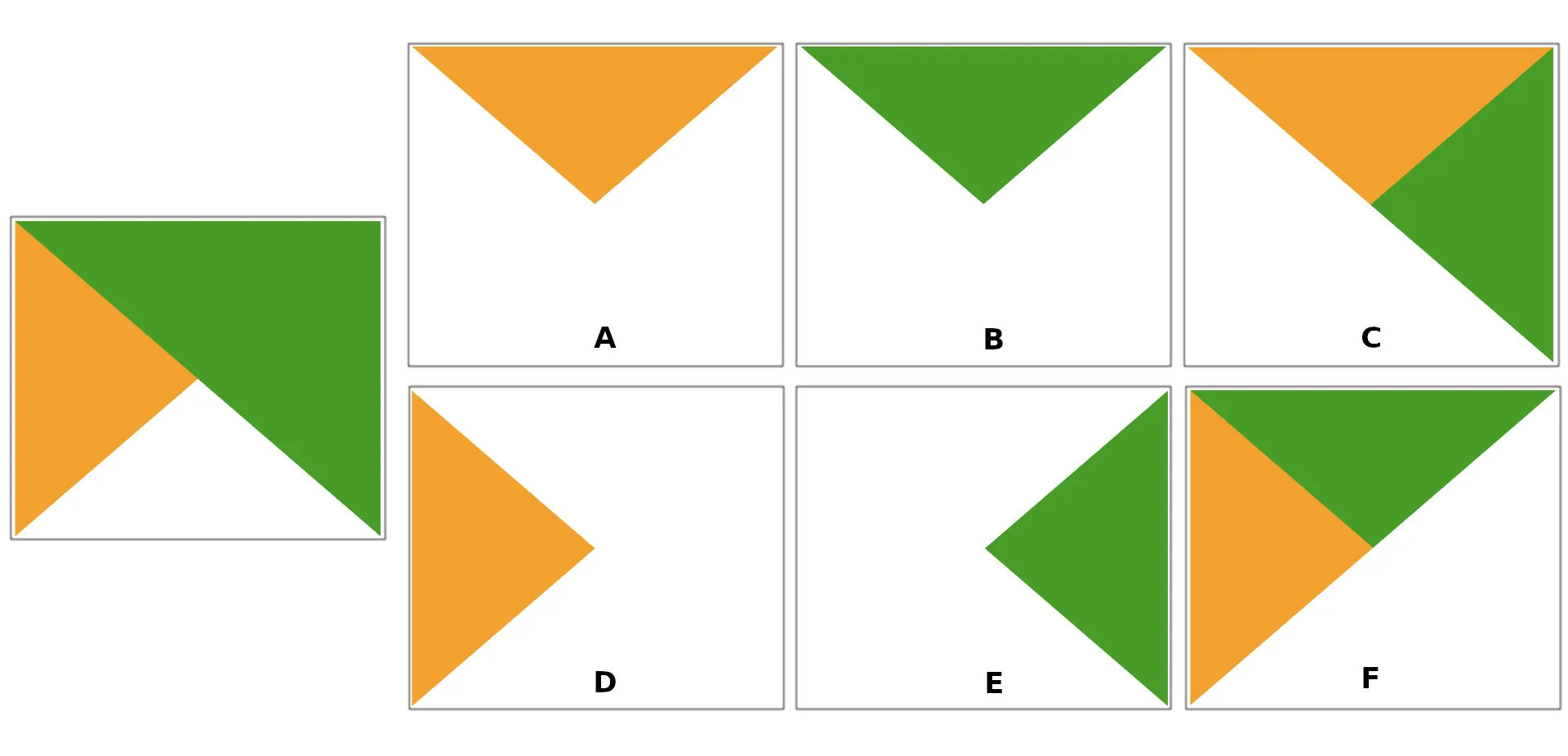
• A: Mask Below
• B: Masked By Below
• C: Paint Below Inside
• D: Inverse Mask Below
• E: Inverse Masked By Below
• F: Paint Inside Below

Blending mode properties are available for both vectors and rasters and can usually be found in the Layer Rendering part at the bottom of the Styling Panel (F7) or Layer Properties ▶ Symbology dialog.

Blending rasters

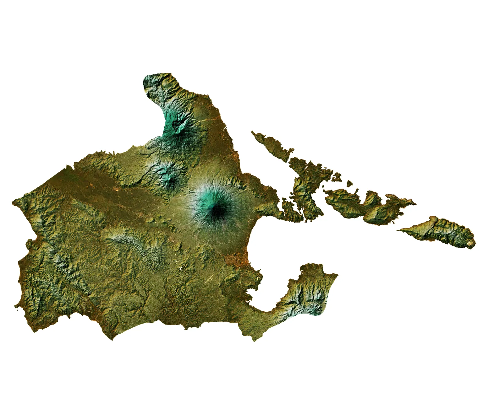
Exercise 2.1.1. Using blending to style rasters

PRO-TIP

For our training participants, you can load the completed/styled layer by loading the blending-modes-raster project found inside bnhr_qgis-advanced-styling.gpkg

In this exercise, we’ll utilize the power of blending modes to style a raster similar to this post: https://bnhr.xyz/2019/01/22/hillshade-in-qgis.html

1. Load the albay_srtm_32651 raster and duplicate the layer.
2. Name the original layer as colored and the duplicate as hillshade pertaining to the style that we will use for the layers. Make sure that the hillshade layer is at the bottom and the colored layer is on top.

Figure 3. Rasters loaded in QGIS

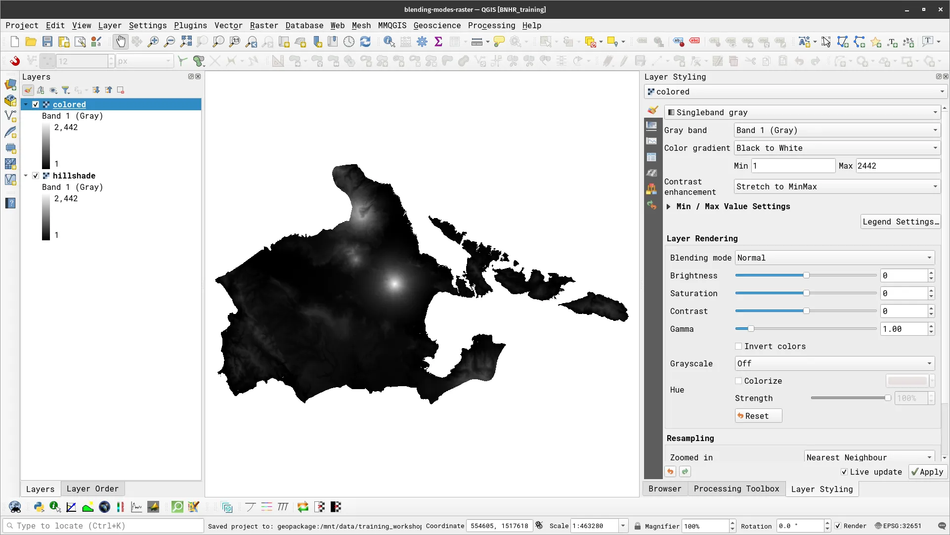
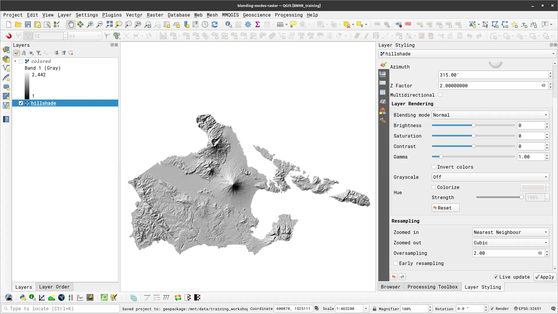
3. Style the hillshade layer with a multidirectional hillshade.
   • Select Hillshade as Render Type
   • Set Z Factor to 2.0
   • Check the Multidirectional checkbox
   • Select Nearest Neighbor and Cubic for Resampling with Oversampling at 2.0
4. The layer should look like the one below.

Figure 4. Hillshade raster styled

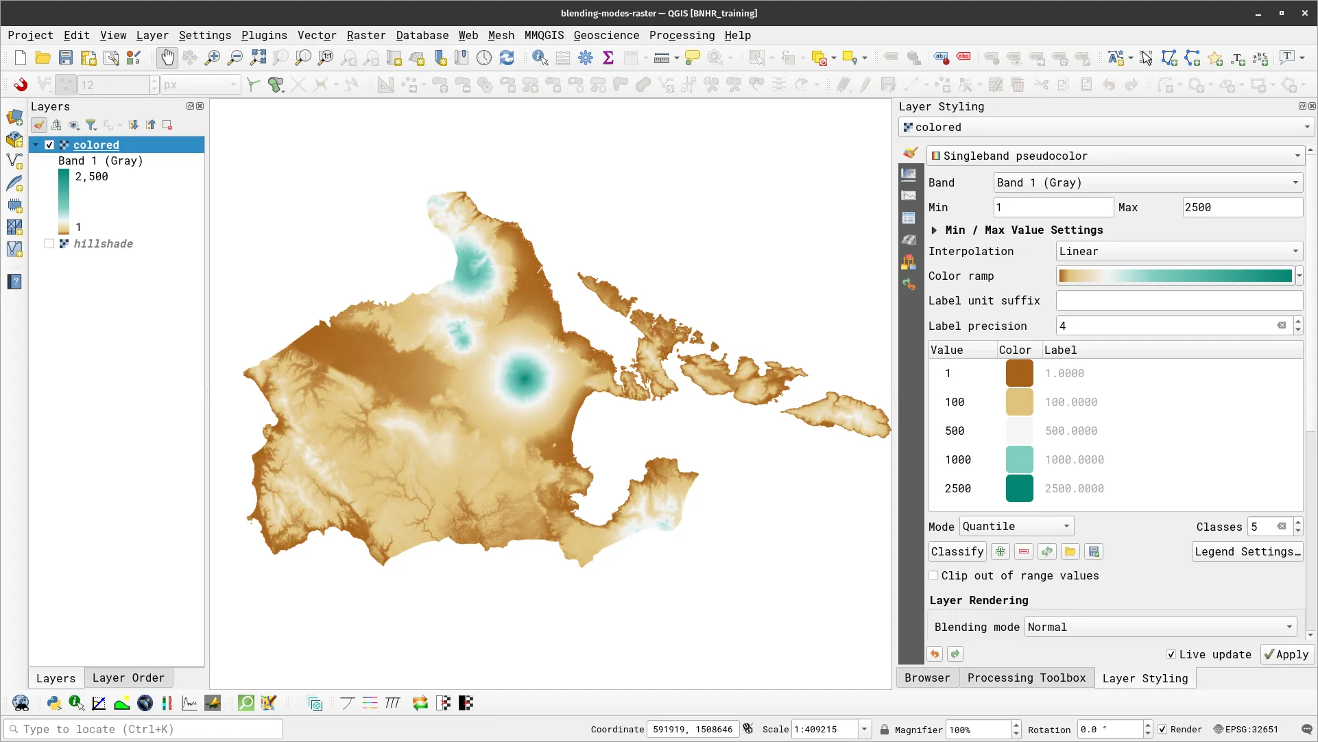
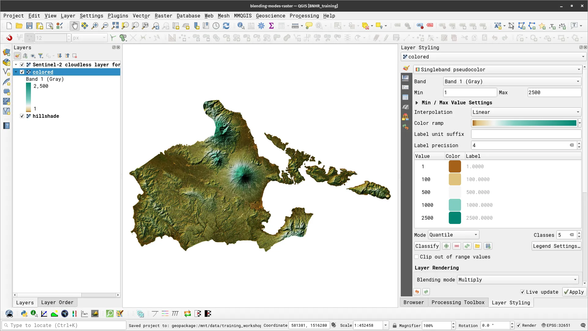
5. Style the colored layer with a singleband pseudocolor symbology.
   • Select Singleband pseudocolor as Render Type
   • For the Color ramp, BrBG works great
   • Edit the Classification intervals (0, 100, 500, 1000, 2000 should work)

Figure 5. Colored DEM layer styled

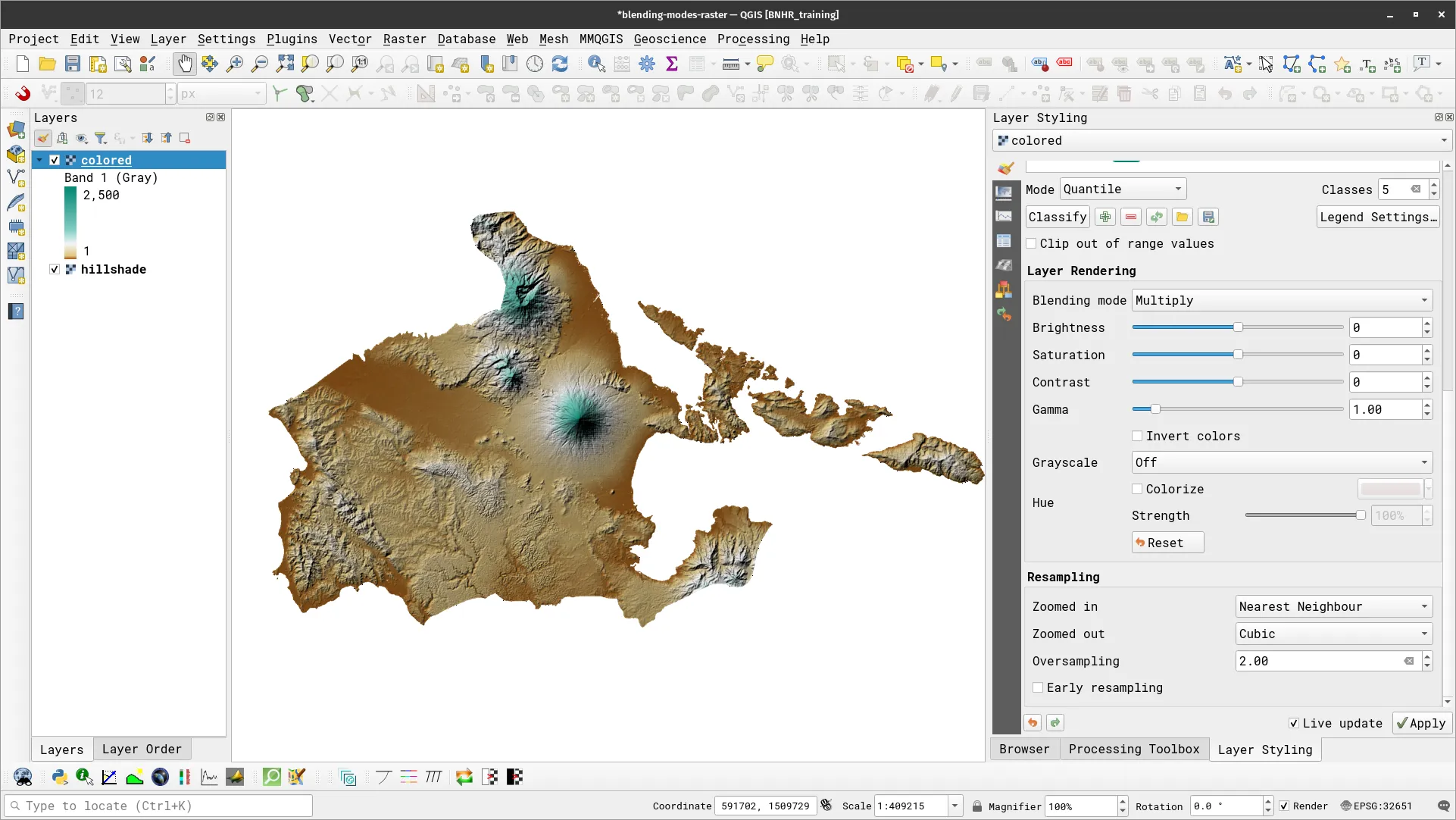
6. Use blending modes.
   • Select Blending mode as Multiply
   • Select Cubic and Average for Resampling with Oversampling at 2.0

Figure 6. Blended (multiplied) colored and hillshade layer

7. Another trick I’ve found is adding/overlaying satellite imagery. For this, load a satellite image (e.g. Bing VirtualEarth or other cloudless satellite imagesy) covering the area.

Figure 7. Satellite imagery loaded in QGIS

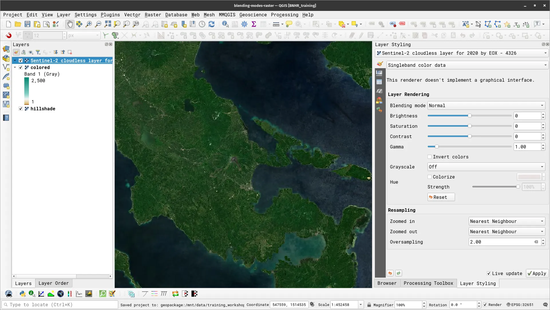
8. Style the satellite image layer. a. Select Blending mode as Overlay b. Update the Brightness, Contrast, and Saturation c. Select Cubic and Average for Resampling with Oversampling at 2.0
9. Your map should look like below.

Figure 8. Combined colored, hillshade, and satellite image layer

Bivariate choropleth maps in QGIS

Bivariate choropleth maps are both stunningly beautiful and informative. With the right color combination, a bivariate choropleth map hits that sweet spot of being both visually stunning and easily understandable.

In essence, a bivariate choropleth map is a combination of two choropleth (univariate) maps. What’s a choropleth map? A choropleth map is a thematic map wherein areas (typically geographic areas) are colored, shaded, or patterned based on the value of a single variable (univariate) corresponding to that area. One of the most basic examples is a population density map. A choropleth map can be created in QGIS by using Graduated Symbology on a polygon vector.

When creating choropleth maps (whether univariate or bivariate), it’s important to remember this rule: Use rates/percentages, not counts/totals. Using rates/percentages is important because if we used counts/totals, we’d introduce the bias to our maps brought by the fact that larger areas tend to have higher population. For example, when creating an election map, a candidate can obtain more votes in Metro Manila than Tawi-tawi not because he is more popular in the former but simply because there are more voters in the Metro Manila than Tawi-tawi.

NOTE

If choropleth maps are not normalized they become merely another population map.

A bivariate choropleth map is similar to a basic (univariate) choropleth map but instead of a single variable, it shows (surprise surprise) two variables at once. A bivariate choropleth map doesn’t just show two variables at once but it also shows a relationship between these two variables—do they agree or disagree, do they increase/decrease proportionally, etc.

Since a bivariate choropleth map shows two variables, the number of categories it has increases exponentially by two – a bivariate choropleth using two univariate choropleth with 3 categories each has 9 categories.

PRO-TIP

Having too many categories in a single map isn’t good practice so a 3x3 or 4x4 bivariate choropleth is workable but anything above that is usually too much.

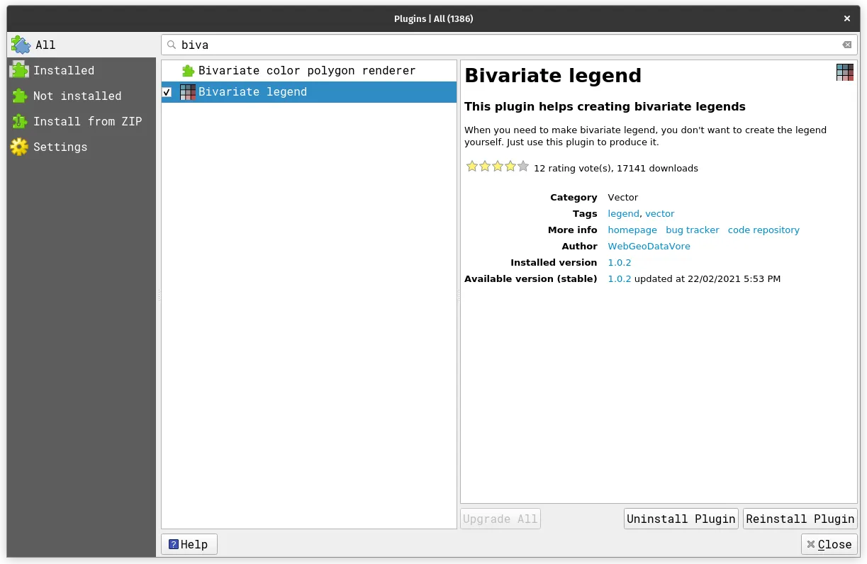
There are several ways to create bivariate choropleth maps in QGIS. For example there is the Bivariate color polygon renderer plugin that adds a bivariate choropleth renderer in the QGIS styling panel. In the next exercise, we will take a more manual approach to creating these kinds of maps in QGIS by utilizing blending modes. We will create a bivariate choropleth map in QGIS similar to the one done in this post: https://bnhr.xyz/2019/09/15/bivariate-choropleths-in-qgis.html

Exercise 2.1.2. Using blending for bivariate choropleth maps

PRO-TIP

For our training participants, you can load the completed/styled layer by loading the blending-modes-bivariate project found inside bnhr_qgis-advanced-styling.gpkg

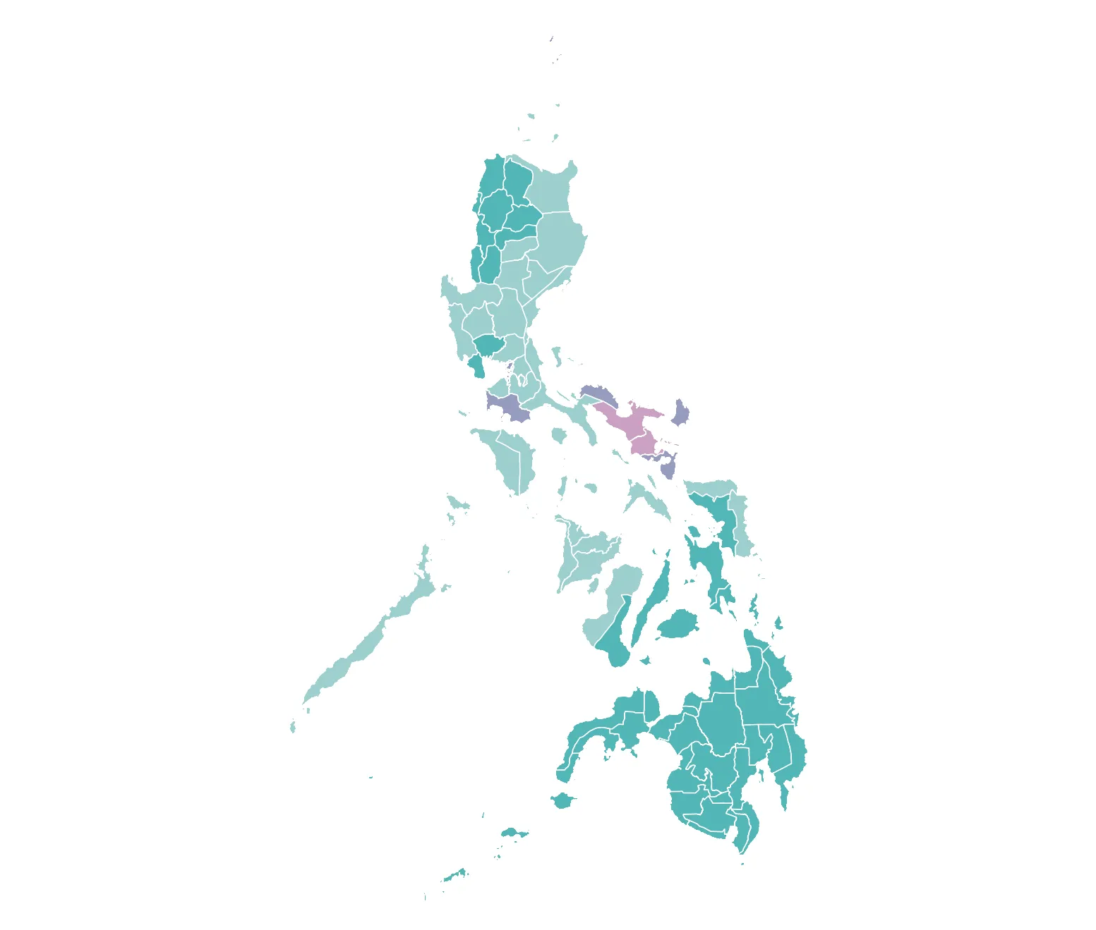
1. Load the 2019_elections_bato_chel data inside bnhr_qgis-advanced-styling.gpkg

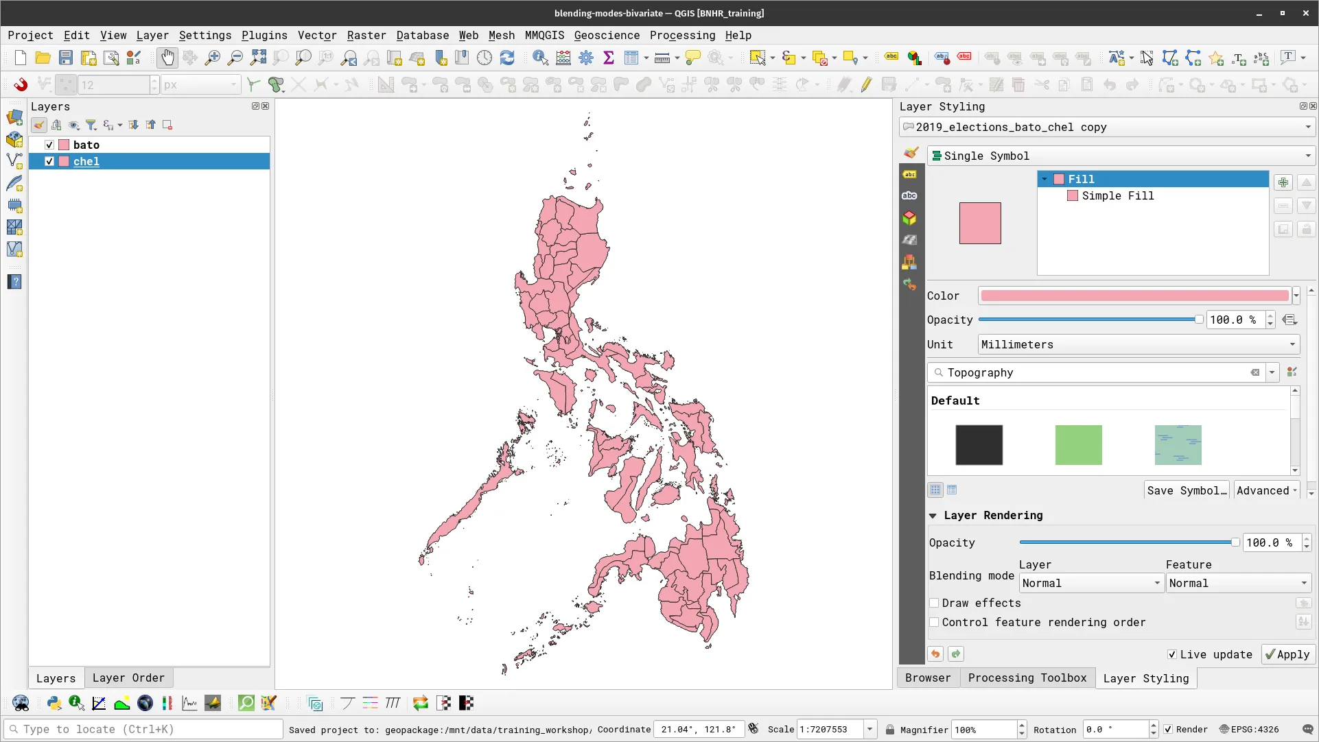
2. Duplicate the layer. Since we’ll be creating a bivariate choropleth map, we need 2 vector layers to show. In this case, we’ll show the percentage of total votes obtained by Bato and percentage of total votes obtained by Chel per province. As such, name the layers bato and chel.

Figure 9. bato and chel layers in QGIS

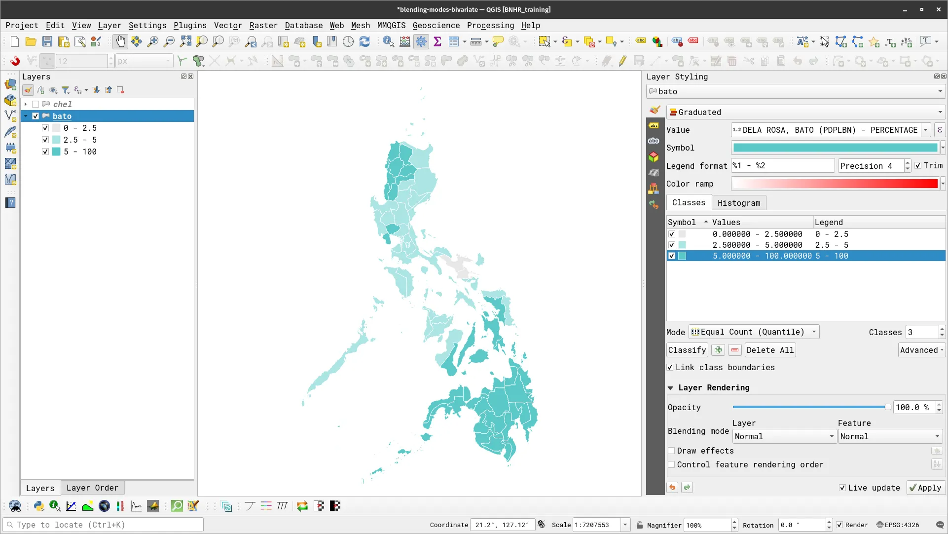
3. Next, we make a choropleth map for the bato layer.
   • Symbology: Graduated
   • Column: DELA ROSA, BATO (PDPLBN) - PERCENTAGE
   • Classes
     • 0.0 - 2.5
       • Color: #e8e8e8
       • Values: 0.000 - 2.5000
     • 2.5 - 5.0
       • Color: #ace4e4
       • Values: 2.500 - 5.000
     • 5.0 - 100
       • Color: #5ac8c8
       • Values: 5.000 – 100.000

Figure 10. Style parameters for bato layer

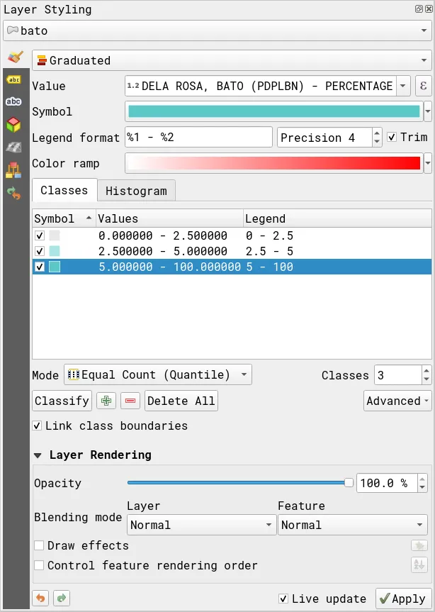
4. Your bato layer should look like:

Figure 11. Choropleth map for bato layer

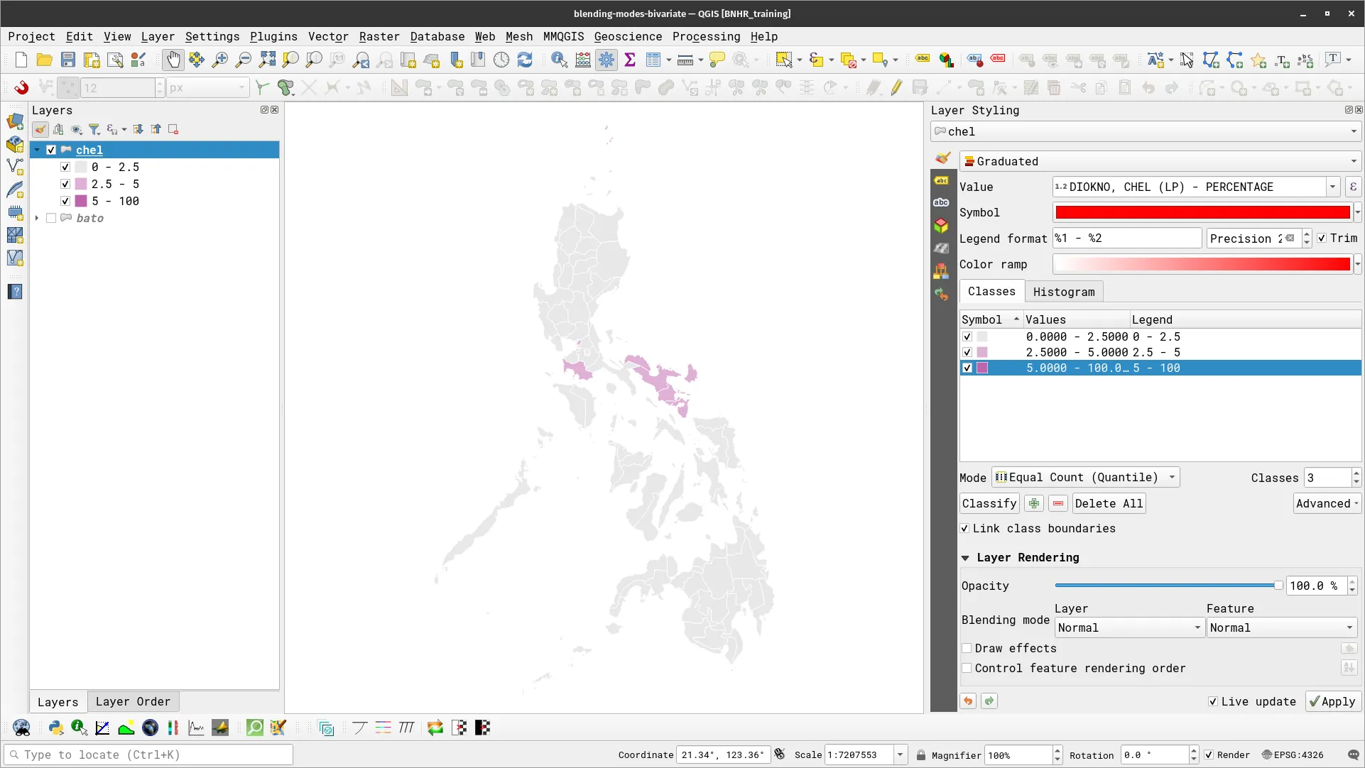
5. For the chel layer, our parameters will be:
   • Symbology: Graduated
   • Column: DIOKNO, CHEL (LP) – PERCENTAGE
   • Classes
     • 0.0 - 2.5
       • Color: #e8e8e8
       • Values: 0.000 - 2.5000
     • 2.5 - 5.0
       • Color: #dfb0d6
       • Values: 2.500 - 5.000
     • 5.0 - 100
       • Color: #be64ac
       • Values: 5.000 – 100.000

Figure 12. Style parameters for chel layer

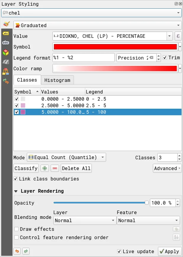
6. Your chel layer should look like:

Figure 13. Choropleth map for chel layer

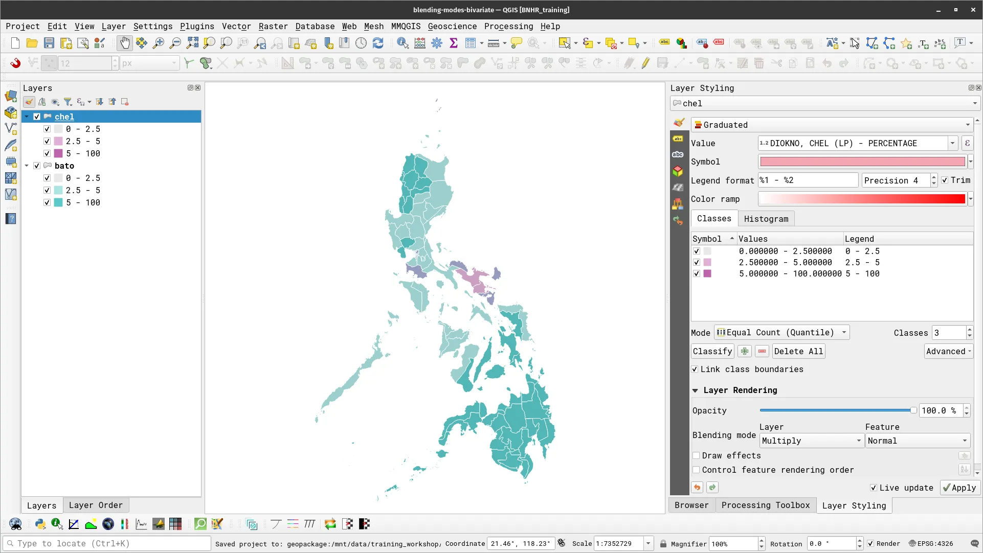
7. Now that you have the two choropleth maps, create the bivariate choropleth effect by changing the blending mode of the top layer (chel) to Multiply.

Figure 14. Bivariate choropleth of the percentage of votes per province garnered by Bato and Chel

PRO-TIP

You can use the Bivariate legend plugin to create a legend for the map you created.

Figure 15. The Bivariate legend plugin

Emphasizing density with Feature-level blending

In the previous exercise, we used blending at the layer level by blending two layers. However, we can also apply blending to work at a level of a layer’s individual features. This approach is particularly useful when we want to emphasize density (or de-emphasize sparseness) especially for feature-rich data with multiple overlapping geometries such as roads.

Exercise 2.1.3. Using blending to emphasize features

PRO-TIP

For our training participants, you can load the completed/styled layer by loading the blending-modes-feature project found inside bnhr_qgis-advanced-styling.gpkg

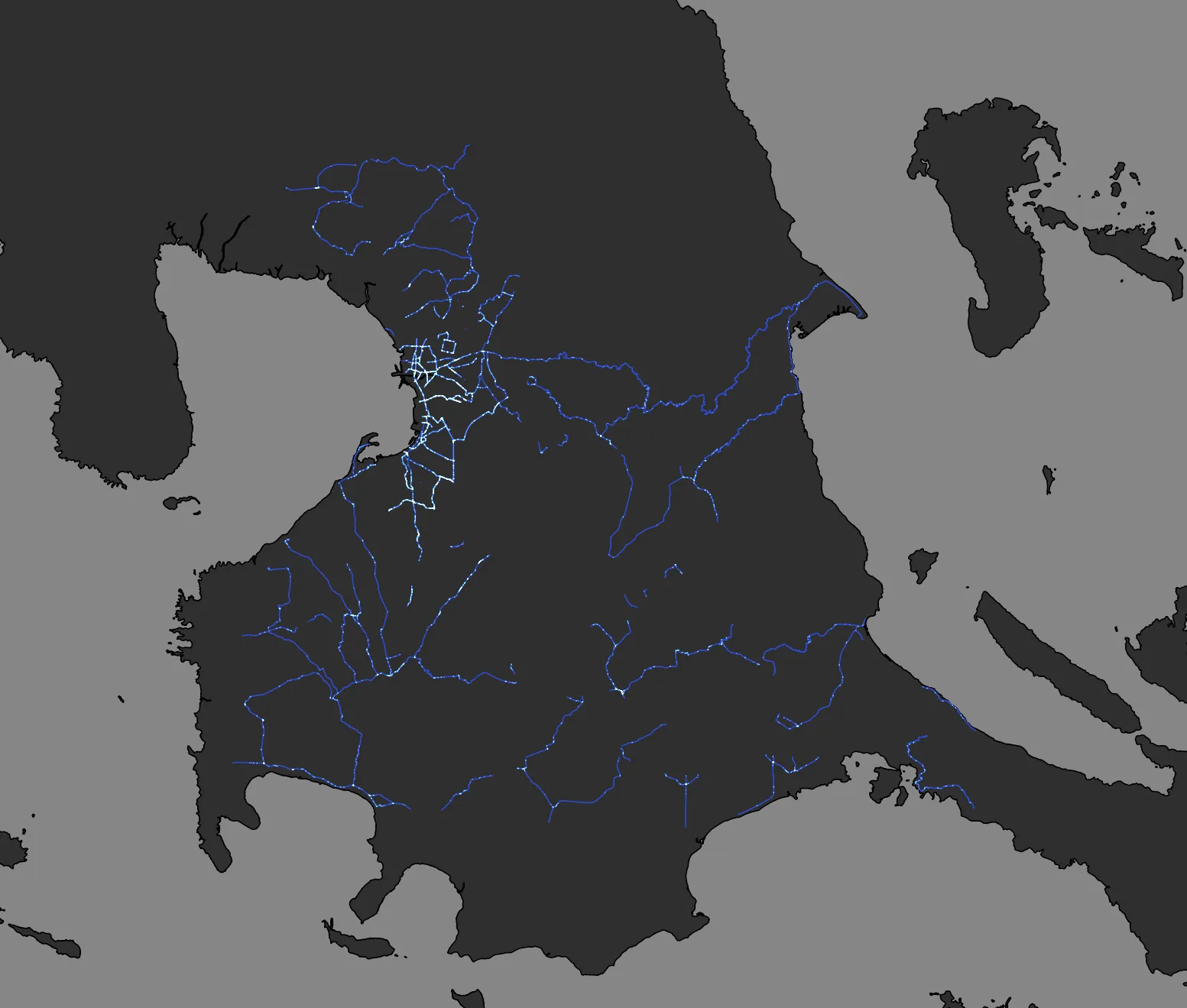
In this exercise, we will highlight areas with dense road densities using a simple feature blending technique.

1. Load the phl_country vector layer and style it as all black (#000000) or any dark color. This will make for a great basemap for our glowing road density map.

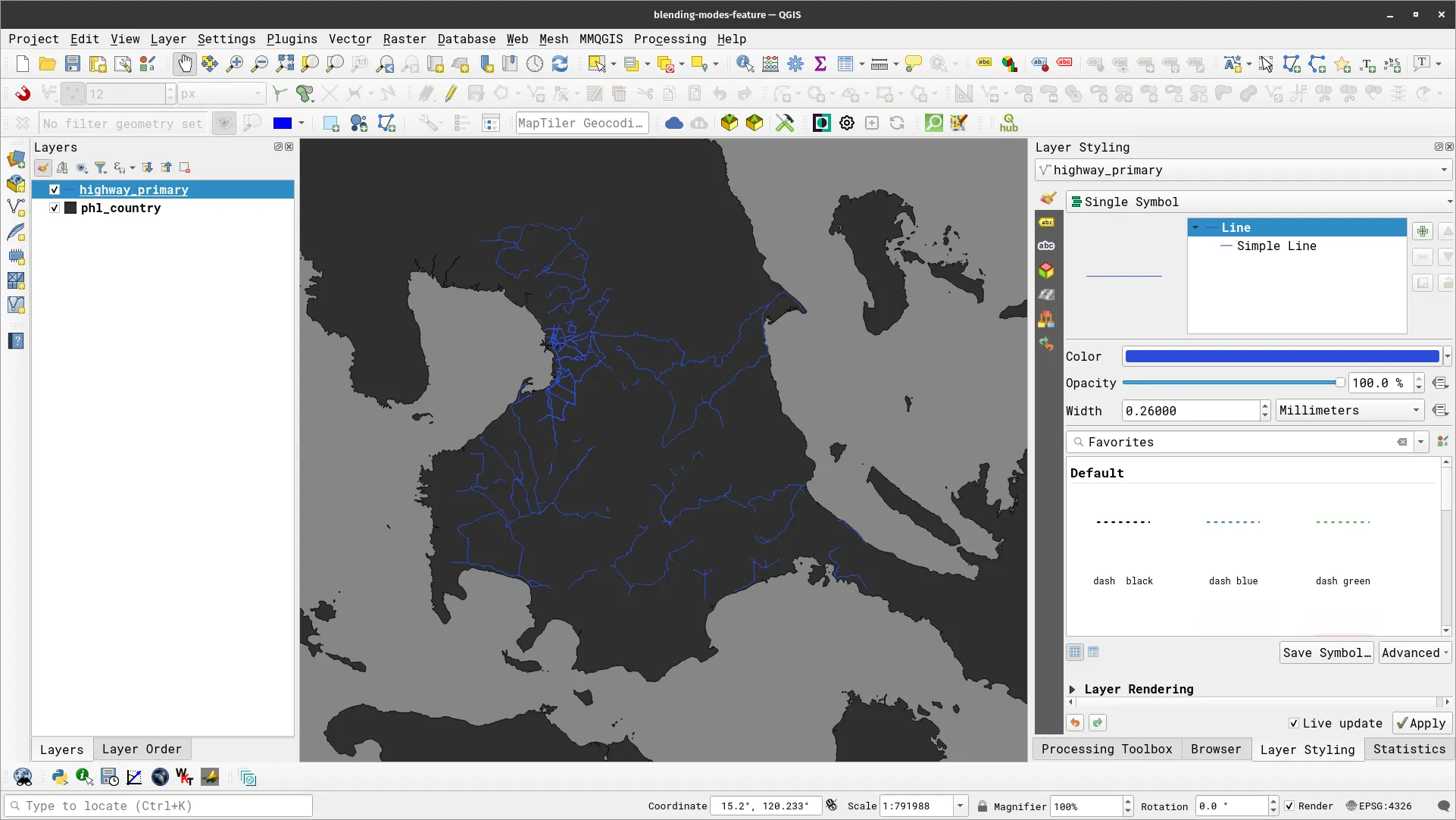
2. Load the highway_primary vector layer. This layer consists of highways/roads tagged as primary from OSM. Style Style this to use blue (#2d4cd9) as its color. As you might notice, the road layer appears dull.

Figure 16. The road layer looks dull and areas with dense road networks aren’t emphasized

3. We will use a simple trick to make this map glow and emphasize the areas with dense road networks. Under the Layer Rendering options of the highway_primary layer, select Addition for the Blending mode under Feature.

Figure 17. The road layer with Addition blending mode on its features

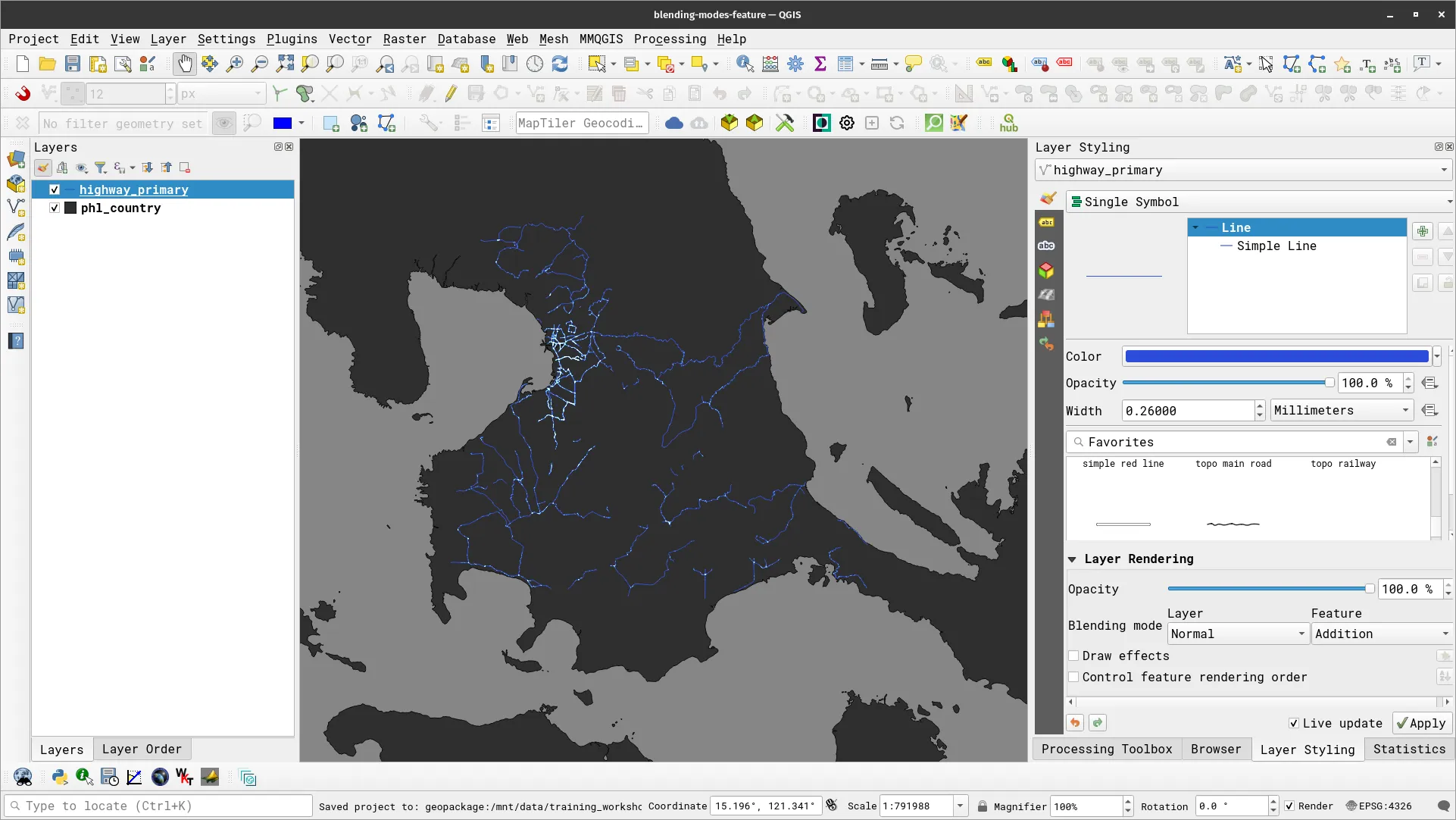
4. Try to play around with line width, color, transparency., and other styling combinations to see what works best for you.

Geometry generators and Expressions

We discussed how to use geometry generators and expressions in the QGIS: Expressions module. Geometry generators allow you to create new geometries using QGIS expressions and existing geometries. This means that we can create polygon, lines, and point geometries without the need for creating new layers. For example, you can generate a buffer geometry from a point layer or a centroid geometry from a polygon layer. Geometry generators also allow us to create complex geometries and styles.

When working with geometry generators, it is important to remember that the correct geometry type has to be set in order for the geometry generator to work. If the final geometry is a point (e.g. centroid) select Point/Multipoint as the geometry type. If it is a polygon (e.g. buffer), select Polygon.

Exercise 2.2. Styling polygons as points/circles

PRO-TIP

For our training participants, you can load the completed/styled layer by loading the geom-generators-expressions project found inside bnhr_qgis-advanced-styling.gpkg

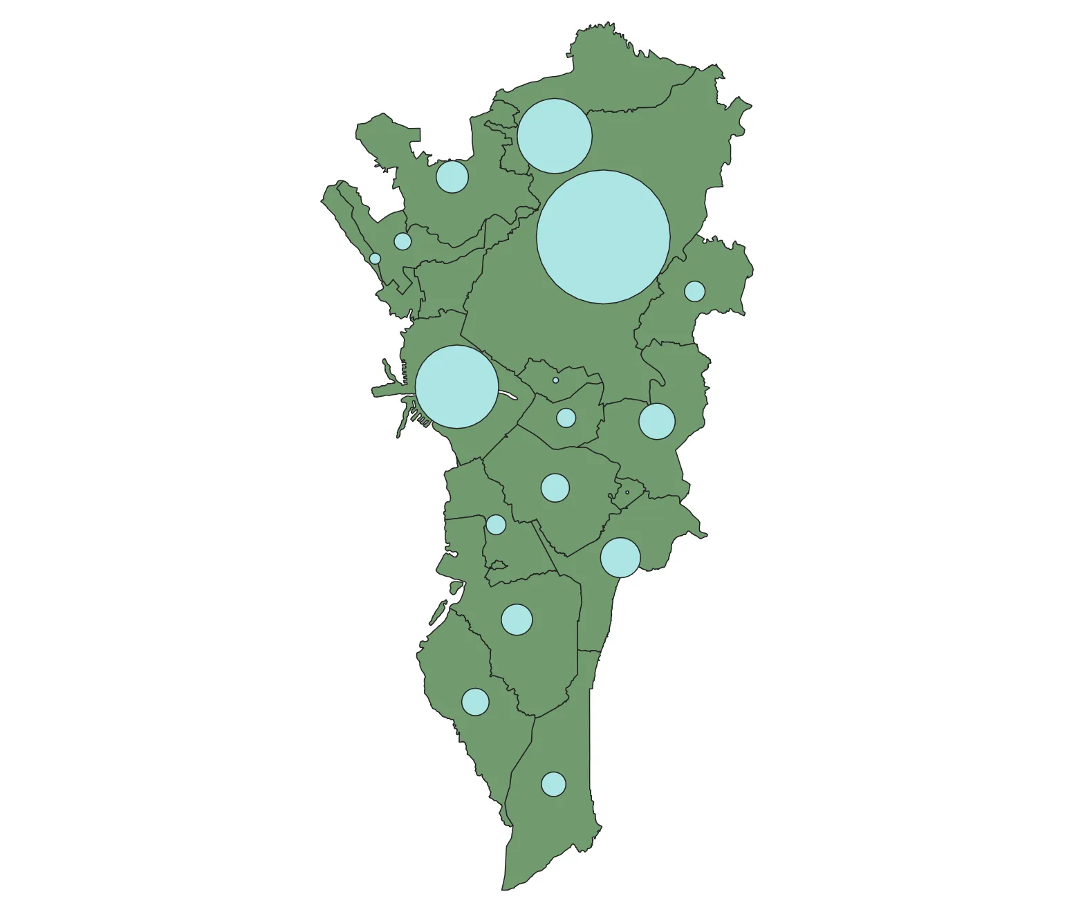
In this exercise, we will style a polygon layer of populations as circles (or more specifically as variable buffers around its centroid where the size of the circle depends on the population in the area).

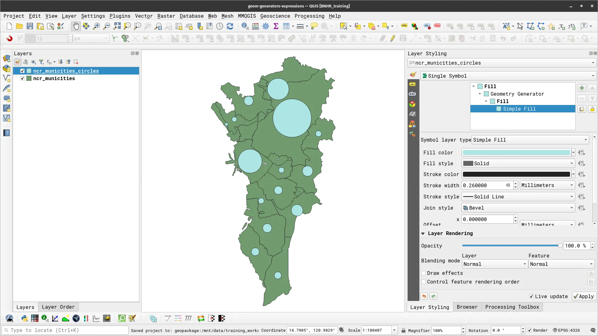
1. Load the ncr_municities layer and duplicate it. Name the duplicate ncr_municities_circles.
2. Apply the following style to the ncr_municities_circles layer.
   • Single Symbol
   • Symbol layer type: Geometry Generator
   • Geometry type: Polygon / Multipolygon
   • Units: Map Units
   • Expression

buffer(centroid($geometry), ("pop2020"/maximum("pop2020"))/30)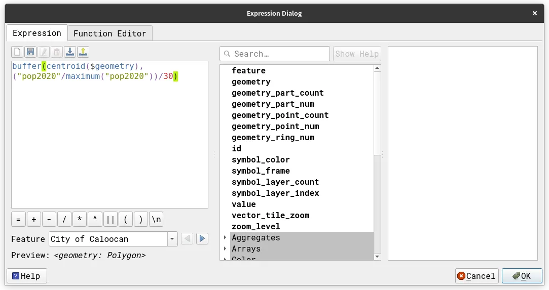

Figure 18. Geometry generator expression for creating a buffer from the centroid of a polygon

3. The expression above creates a buffer around the centroid of the polygon features where the buffer distance is equal to the ratio of the feature’s population to the maximum population in the layer. The “30” is used to scale the size of the circles.

Figure 19. ncr_municities polygon layer styled as variable-size circles

Data-defined overrides

Data-defined overrides are powerful tools in QGIS. Through this mechanism, a user can use dynamic values for styling parameters such as color, size, rotation, etc. A data-defined override is available for a parameter when the data-defined override button appears to its right. Clicking on this button reveals the different options available for the user. The override can be based on:

• A field/attribute value
• A QGIS expression

For an override to work, it must be in the same type as the value it is overriding. For example, a size parameter must be overridden by a number, a color parameter must be overridden by a string pertaining to a color. When a data-defined override is active, the button turns yellow ().

Exercise 2.3. Using both size and color to communicate information

PRO-TIP

For our training participants, you can load the completed/styled layer by loading the data-defined project found inside bnhr_qgis-advanced-styling.gpkg

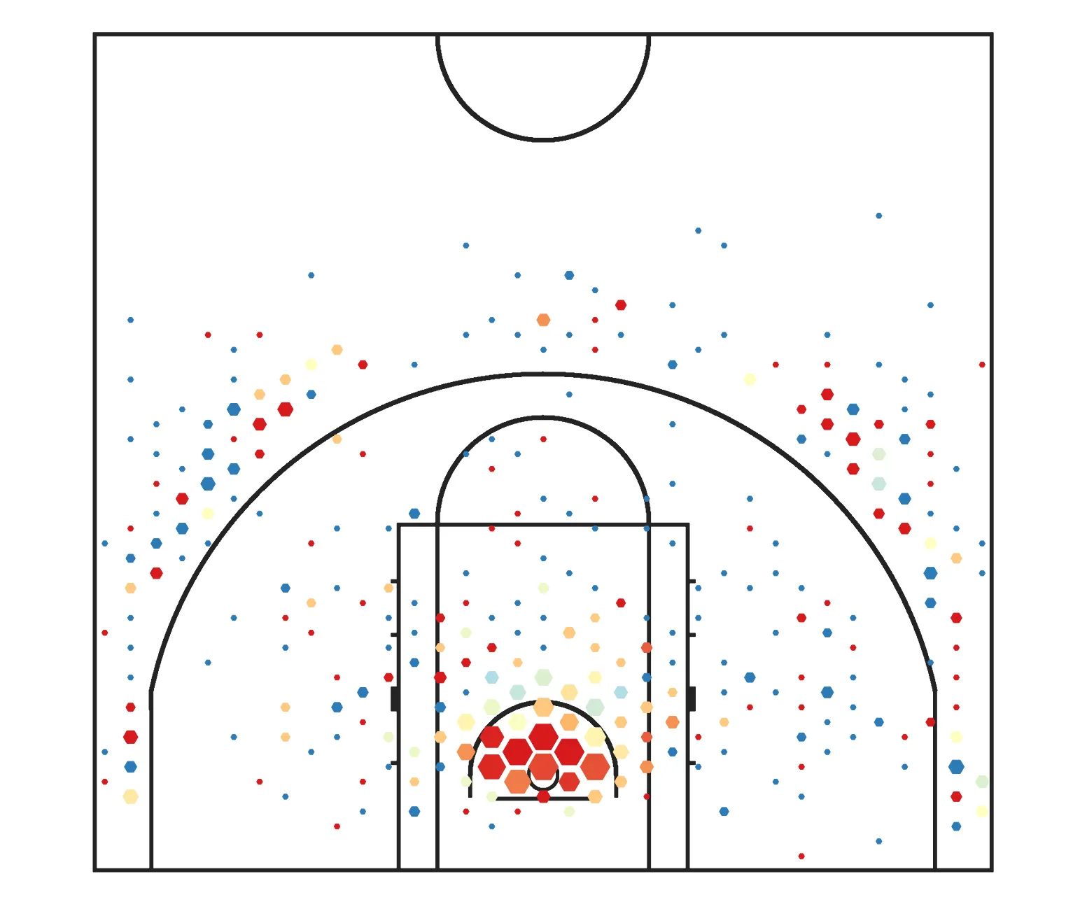
In this exercise, we will use both size and color to communicate information by taking advantage of QGIS’ ability to have these values be dynamic and be defined by data. Our task is to create a simple basketball visualization showing the how many field goals a team takes at a specific location on the court (indicated by the size) and how effective—or how many points per attempt the team scores—at that location (indicated by the color).

1. Load the court and ppa-up-hex layers in QGIS. The court layer is just a basketball court (polygon) while the ppa-up-hex is a hex grid layer (polygon) with the following fields:
   • total_fga – the number of field goals attempted in the area/grid cell
   • total_points – the total number of points scored in the area/grid cell
   • ppa – the points per attempt in the area/grid cell

Figure 20. The court and ppa_up_hex layer loaded in QGIS

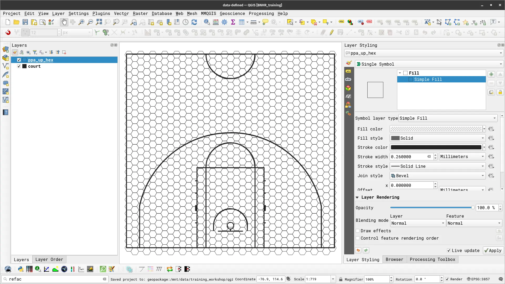
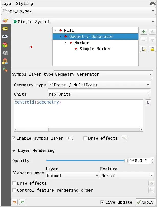
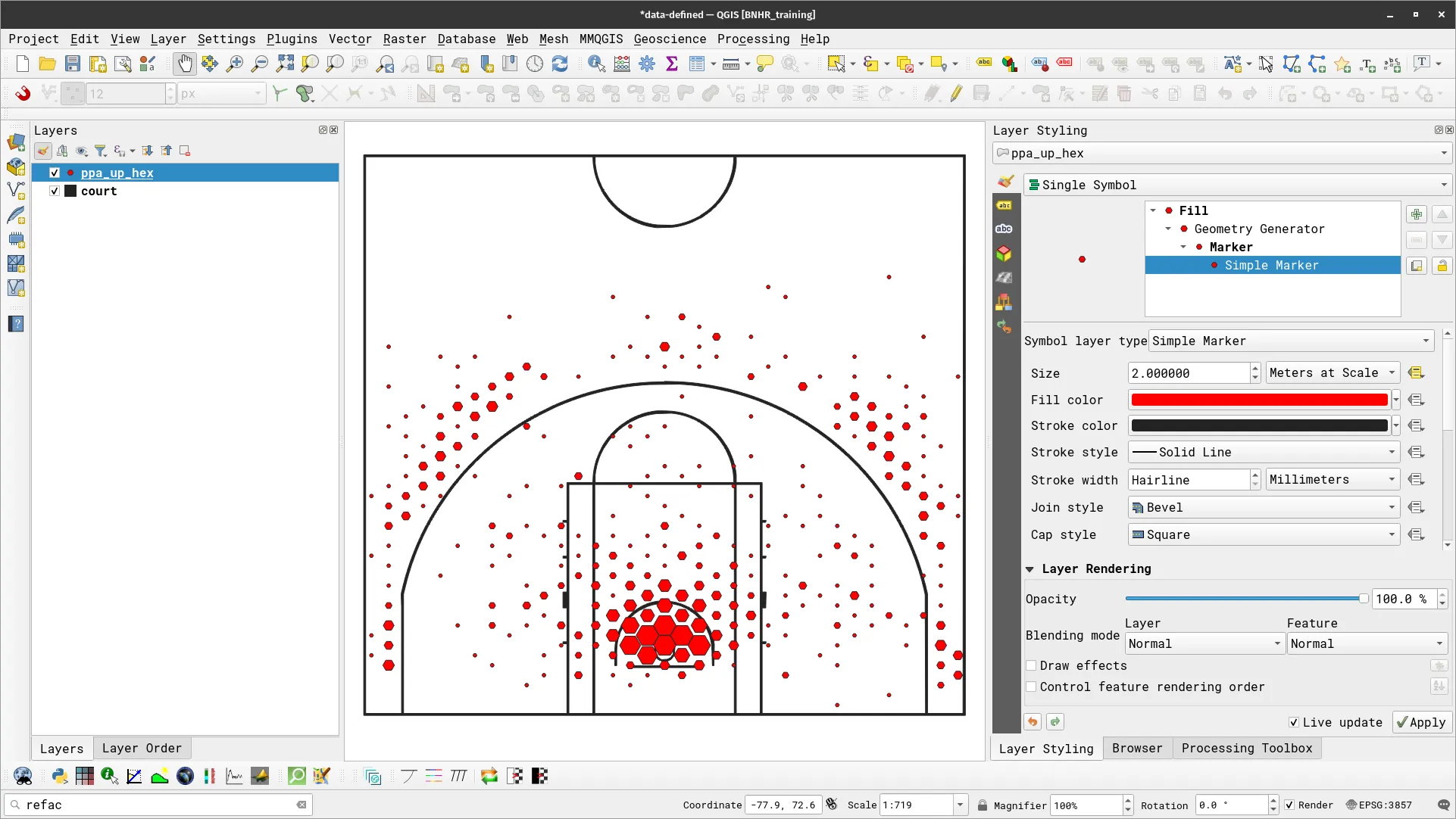
2. Apply a geometry generator symbology to change the grid to a point layer of its centroids.

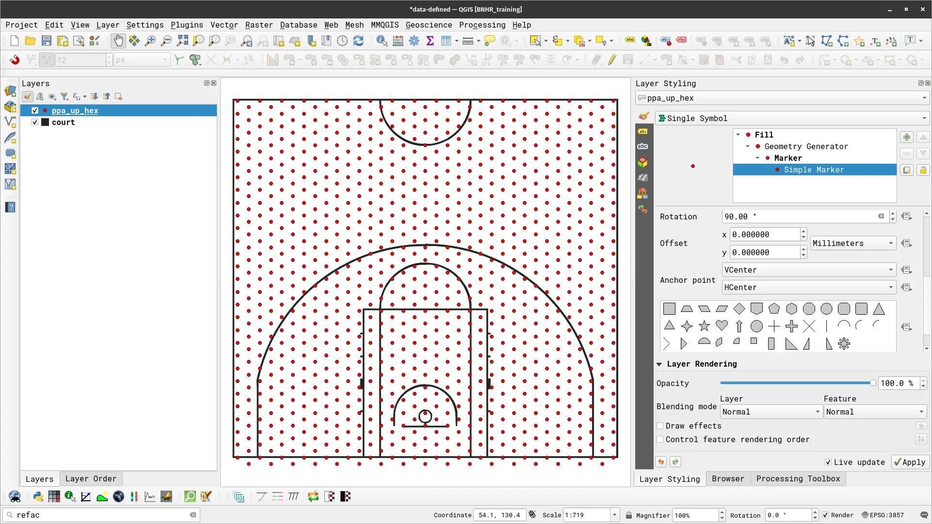
centroid($geometry)

3. Under Simple Marker, change Rotation to 90° and select the hexagon.

Figure 21. Marker options (1)

Figure 22. Marker options (2)

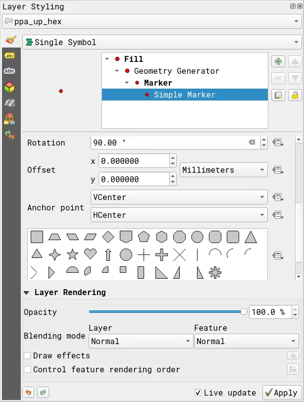
4. Your layers should look like below.

Figure 23. The ppa_up_hex layer styled with hexagonal markers as centroids

5. Now let’s change the size of the marker such that it changes depending on the number of field goals attempted in the location/grid cell it represents. For this, we’ll take advantage of the Assistant to help us. Click the data-defined override button () and select Assistant…

6. The Assistant allows us to easily specify how we want the override the parameter. We simply need to give it the source (can be a field or an expression), the input values, and the output values that we will use for the override. It will then take care of how to convert this into a data-defined override that QGIS can use. In our case, we want to assign the size of a feature (between 1.00 to 5.0 meters) depending on the value its total_fga field (with 1 getting the smallest size and 30+ getting the largest size). Because we want the size in meters, make sure that you have Meters at Scale for the Size units.

Figure 24. Data-defined assistant for the size parameter of the ppa_up_hex layer

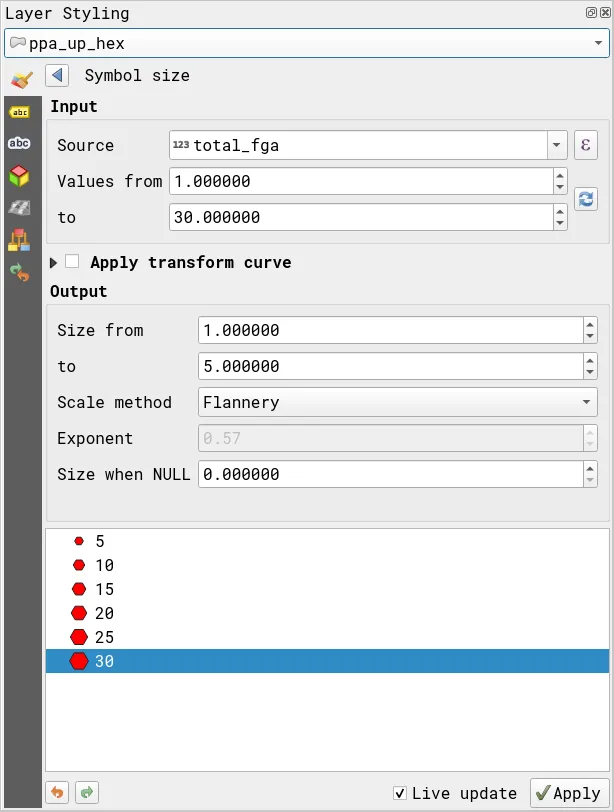
7. Your layer should look like below.

Figure 25. The ppa_up_hex grid with hexagon size showing the number of field goal attempts

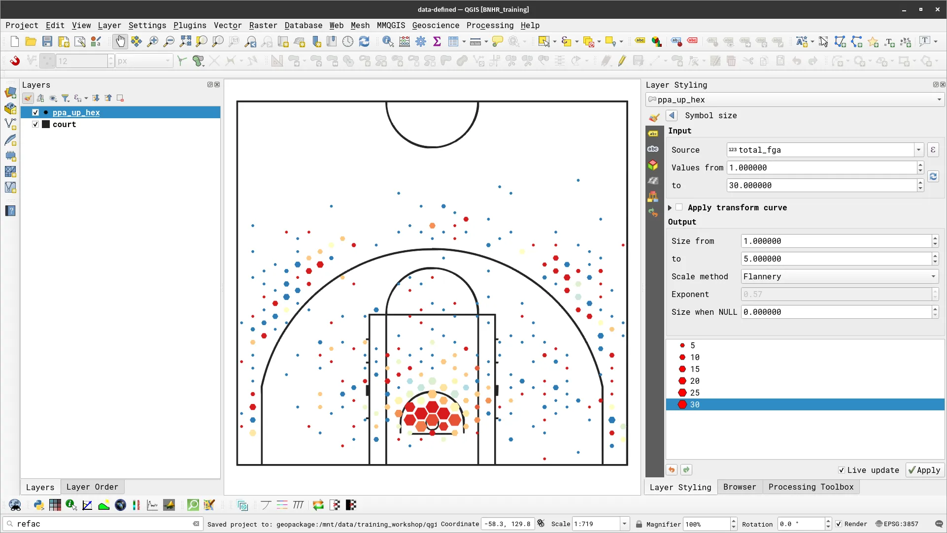
8. Next, let’s have the colors of the hexagon be based on the points scored per attempt at the grid location/cell. To do that, we’ll once again use the Assistant. This time we will change both Fill color and Stroke color. We use the ppa field as source and convert its values (between 0.0 and 1.5) to their corresponding colors in an inverted RdYlBu color ramp with 0.0 pertaining to the left-most color (blue) and 1.50 corresponding to the right-most color (red).

Figure 26. Data-defined assistant for the color parameters of the ppa_up_hex layer

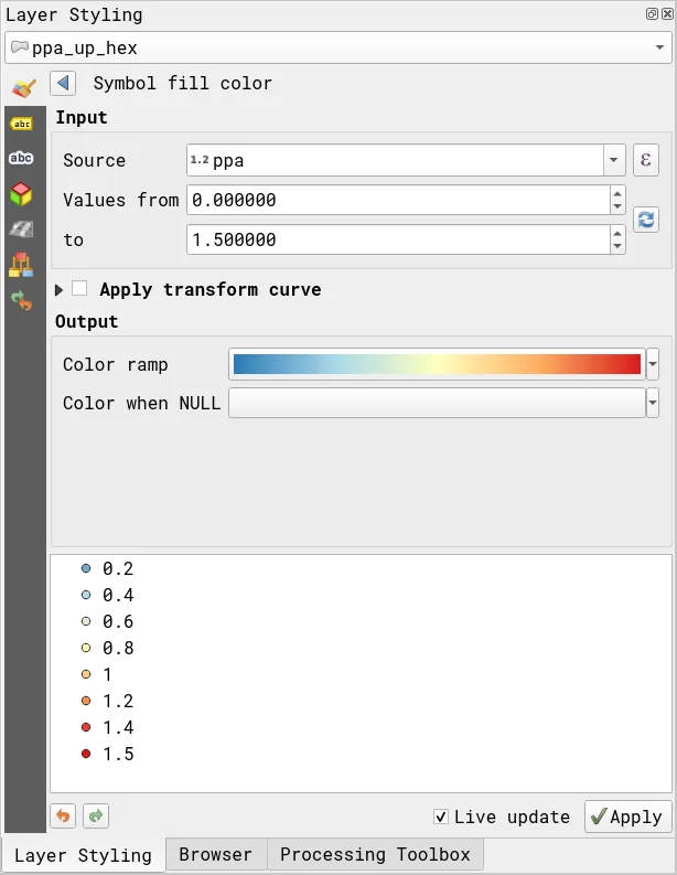
9. We apply the same style to both Fill color and Stroke color.

10. Your layer should now look like below.

Figure 27. The PPA map with size showing the number of field goal attempts in the area and color showing the effectiveness in the area

SOMETHING TO THINK ABOUT

How will you apply a legend in this case?

Draw effects

Since QGIS 2.10, draw effects have been available in QGIS that allows the user to modify and add different effects to the rendering of vectors. These effects can be activated and modified by enabling and clicking the draw effects button (star).

The different effects available to the user are:

• Inner Glow
• Inner Shadow
• Source
• Outer Glow
• Outer Shadow
• Blur
• Colorise
• Transform

The opacity and blend mode can also be modified for each effect. The rendering order of the effects can also be changed via the arrow buttons.

Draw effects are useful for adding glows and shadows to features and layers (i.e. firefly maps).

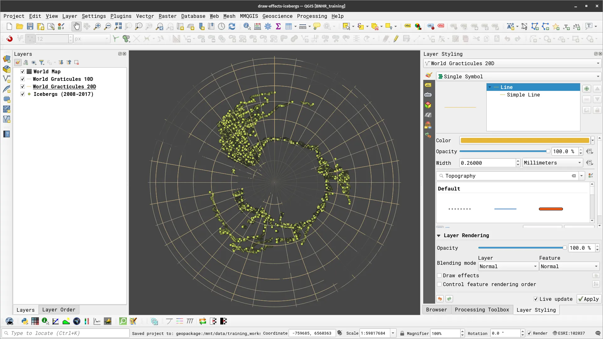
Exercise 2.4. Using Draw Effects to map icebergs

PRO-TIP

For our training participants, you can load the completed/styled layer by loading the draw-effects-icebergs project found inside bnhr_qgis-advanced-styling.gpkg

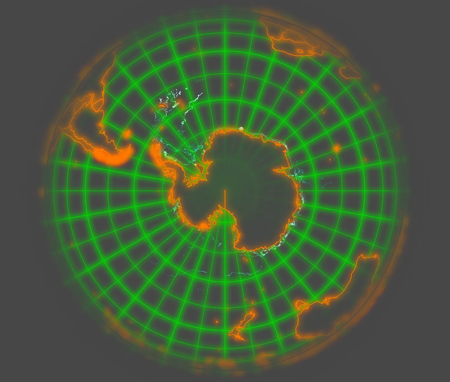
In this exercise, we will use data-defined overrides and draw effects to map icebergs in QGIS similar to this post: https://bnhr.xyz/2019/02/08/mapping-icebergs-in-qgis.html

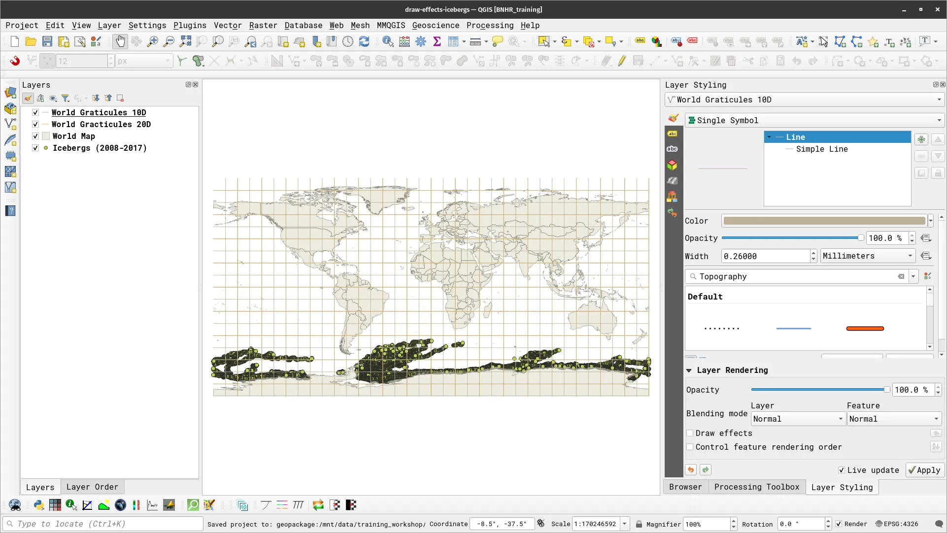
1. Load the Icebergs (2008-2017), World Graticules 10D, and World Graticules 20D vector layers. For a world map, enter world in the coordinate bar of the status bar.

Figure 28. The world, icebergs, and graticule layers loaded in QGIS

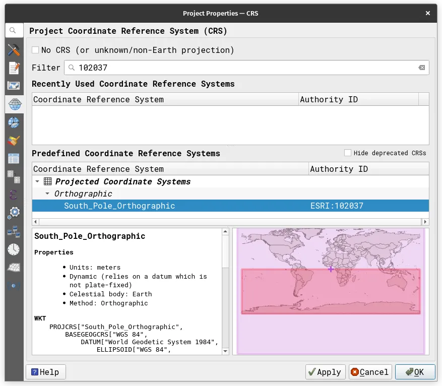
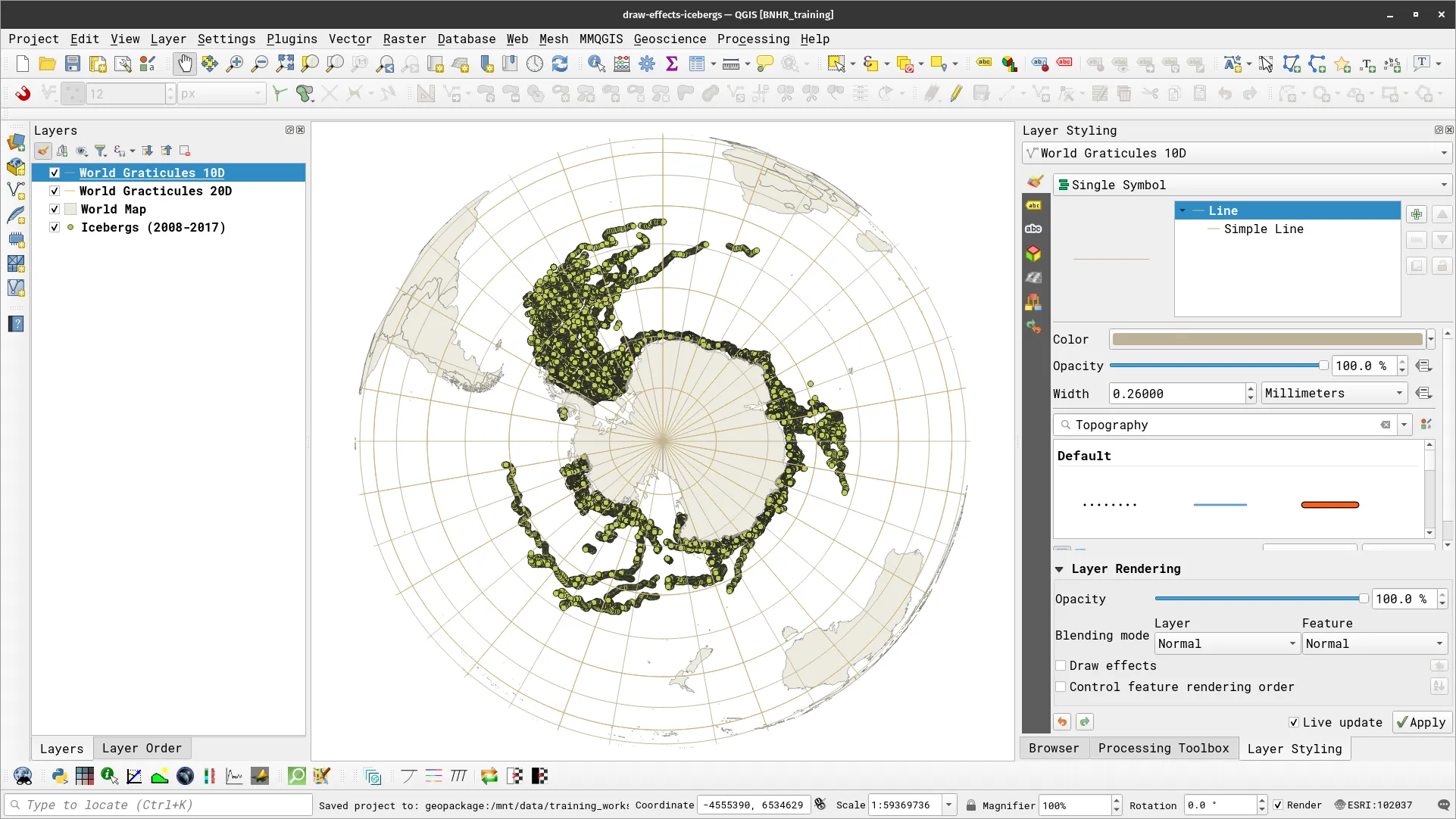
2. First, change the CRS of the project to the South Pole Orthographic projection (ESRI: 102037).

Figure 29. Changing the CRS to South Pole Orthographic

Figure 30. Better looking map using South Pole Orthographic projection

3. Change the Project background color to dark gray (#474747) via Project ▶ Properties ▶ General. Apply a Gradient fill symbology to the world map using #474747 (75% opacity) and #474747 (100% opacity) as the endpoints of a color ramp.

Figure 31. Project background and world map styled

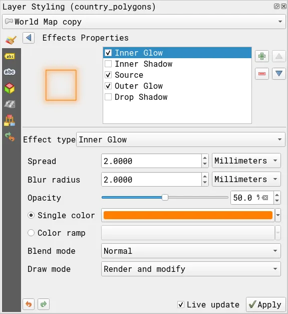
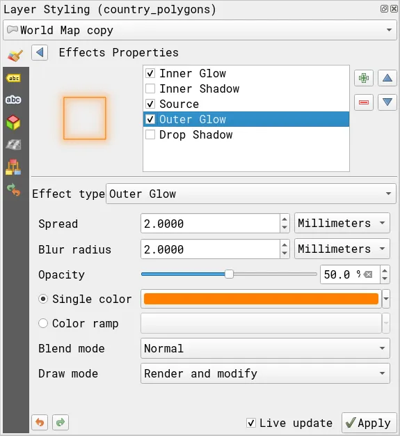
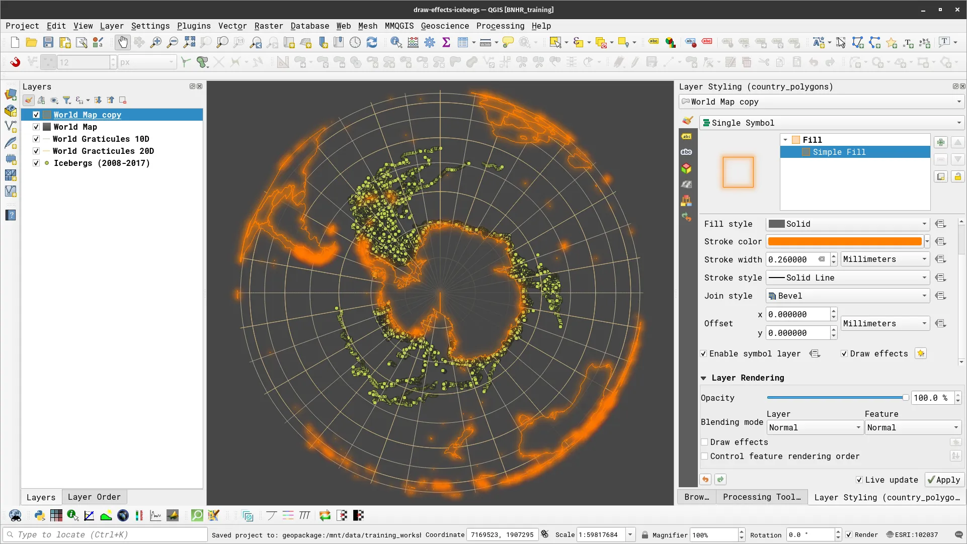
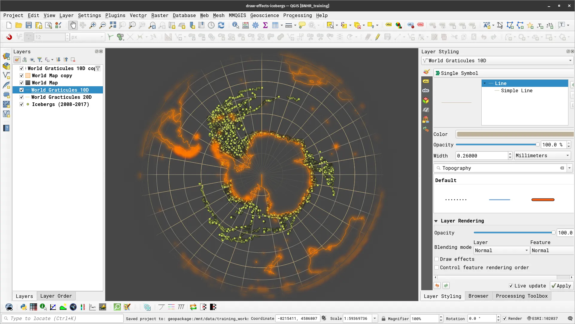
4. Let’s add a glowing effect to the coasts using Draw effects.
   1. Duplicate the World layer.
   2. Select Simple fill as Symbol layer type
   3. Set Fill color to transparent
   4. Set Stroke color to dark orange (#ff7f00)
   5. Check Draw effects under Layer Rendering
   6. Add an Inner Glow and Outer Glow effect with the following properties:
      1. Color: dark orange (#ff7f00)
      2. Spread: 2 mm
      3. Blur radius: 2 mm

Figure 32. Inner glow draw effect for World Map duplicate

Figure 33. Outer glow draw effect for World Map duplicate

Figure 34. World map duplicate with inner and outer glow draw effects

5. Duplicate the World Graticules 10D layer and filter using “display” = ‘10 S’. We’ll use this layer to create the blackish effect around our map. Put this as the first layer in the layer panel.
   1. Select Simple line as Symbol layer type
   2. Set Stroke color to dark gray (#474747)
   3. Check Draw effects under Layer Rendering
   4. Add an Inner Glow and Outer Glow effect with the following properties:
      1. Color: dark gray (#474747)
      2. Spread: 10 mm
      3. Blur radius: 10 mm

Figure 35. Outermost graticule styled to blur the edges of the map

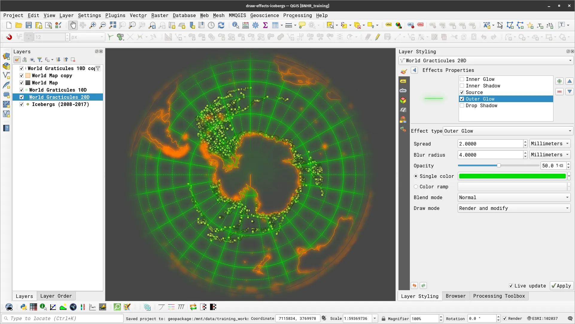
6. Style the World Graticule 20D layer. 

   1. Select Simple line as Symbol layer type
   2. Set Stroke color to green (#02db00)
   3. Select Solid line as Stroke style
   4. Check Draw effects under Layer Rendering
   5. Add an Outer Glow effect:
      1. Color: green (#02db00) with 50% Opacity.
      2. Spread: 2 mm
      3. Blur radius: 4 mm

7. Style the World Graticule 10D layer. 

   1. Select Simple line as Symbol layer type
   2. Set Stroke color to green (#02db00)
   3. Select Dashed line as Stroke style
   4. Check Draw effects under Layer Rendering
   5. Add an Outer Glow effect:
      1. Color: green (#02db00) with 50% Opacity.
      2. Spread: 2 mm
      3. Blur radius: 4 mm

Figure 36. World graticules styled with green firefly/glow effect

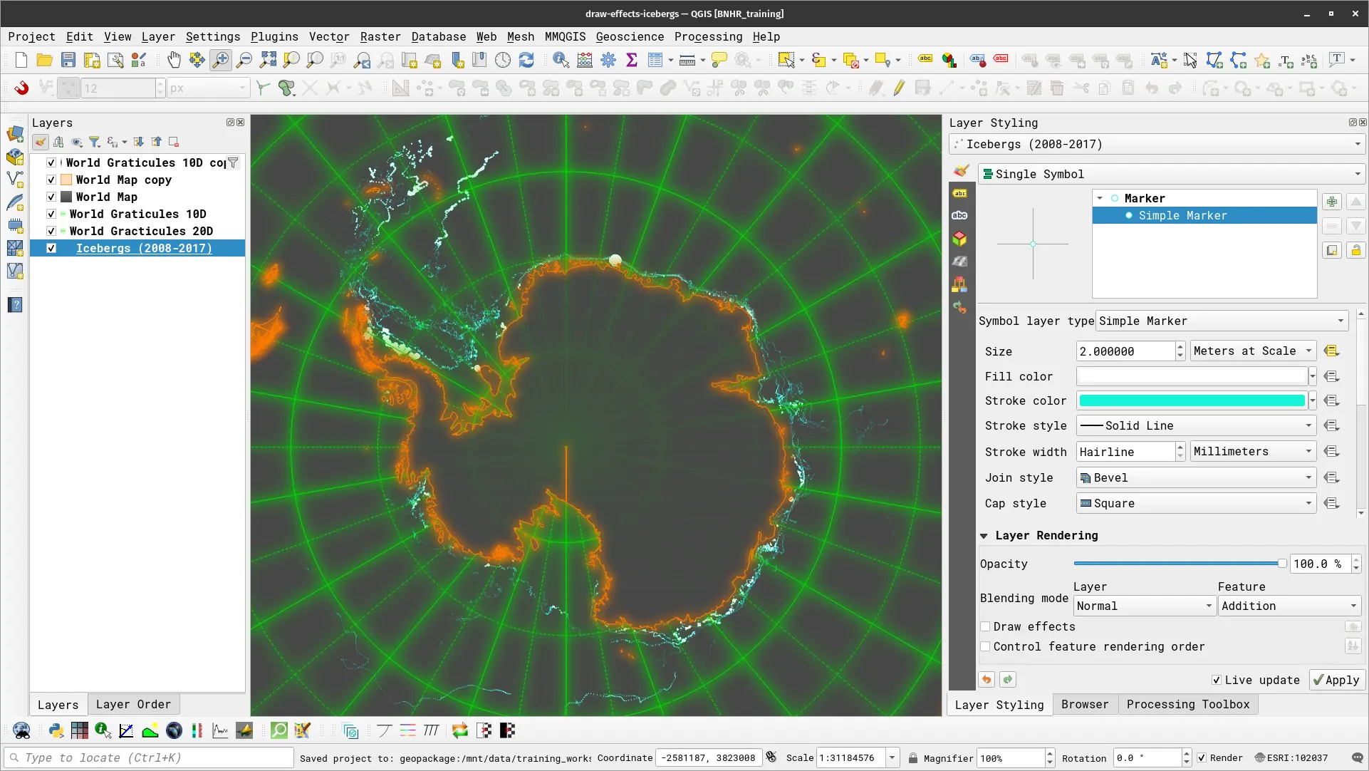
8. For the icebergs layer,
   1. Select Simple marker as Symbol layer type
   2. Use data-defined override to have the size of each iceberg be based on their actual size in real life by using the size field.
   3. Set Fill color to white
   4. Set Stroke color to cyan (#16f3d6)
   5. Finally, instead of using draw effects for glows, you can try the feature-level addition blending mode to highlight areas with lots of icebergs.

Figure 37. Icebergs styled with data-defined size

Figure 38. Iceberg glowing effect using feature-level blending mode

SOMETHING TO THINK ABOUT

Notice that the icebergs layer has a field/attribute pertaining to date, what do you think we can do with that information?

Raster Attribute Table

In version 3.30, QGIS introduced native support for Raster Attribute Tables (RAT). RATs provide the following functionalites:

1. Automatic raster styling: when a raster with an available RAT and style information is loaded in QGIS, QGIS automatically applies the corresponding styles to the raster layer. This functionality works for both embedded RATs and sidecar VAT.DBF files with matching basenames.
2. RAT reclassification: you can reclassify rasters based on different columns.
3. RAT identify: you can identify the pixels that correspond to specific rows.
4. RAT properties: you can view the attribute table of a raster.
5. Raster editing, creation, and classification: RATs can be created from existing paletted or singleband pseudocolor styles and edited accordingly.

Learn more at: https://qgis.org/en/site/forusers/visualchangelog330/index.html#feature-raster-attribute-tables-rat-suppport

Exercise 2.5. Styling a raster using a Raster Attribute Table

PRO-TIP

For our training participants, you can load the completed/styled layer by loading the raster-attribute-table project found inside bnhr_qgis-advanced-styling.gpkg

1. Load a raster layer and preferably one that can be styled as paletted/unique values or singleband pseudocolor symbology. For example, you may refer to Exercise 4.4.2 in the QGIS: Essentials Module 4.
2. After adding your paletted/unique values or singleband pseudocolor, right-click on the layer in the Layers panel > Create Raster Attribute Table. You may choose to save the Raster Attribute Table either:
   1. Managed by the data provider, or
   2. Sidecar VAT.DBF file. NOTE: The VAT.DBF file should have the same name as the raster file that it pertains to.

NOTE

The VAT.DBF file should have the same name as the raster file that it pertains to.

Figure 39. Create new Raster Attribute Table

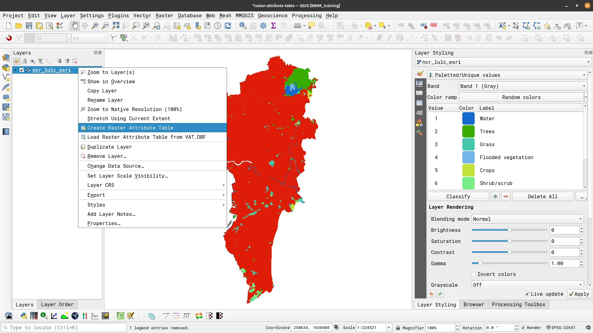
3. It should open the raster attribute table.

Figure 40. The Raster Attribute Table

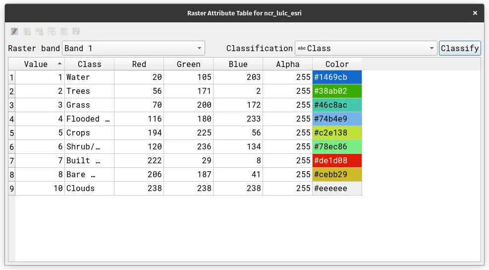
4. If a raster has a Raster Attribute Table assigned to it, it will use the style defined by the RAT when loaded in QGIS. You can open the assigned RAT by right-clicking on the layer > Open Raster Attribute Table.

Certification and support

LOOKING FOR CERTIFICATION AND SUPPORT?

We offer additional resources, certificates, official QGIS certification, ongoing support, and other perks to those who avail of our paid courses.

Contact us or sign-up to our courses if you are interested in having this as an instructor-led or self-paced course.