Beyond 2D and static maps

Introduction

QGIS is powerful data visualization engine not just for conventional maps but also for other data types and visualizations. For example, QGIS has native support and plugins that handle 3D visualizations, point clouds, mesh datasets, and temporal data.

In this module, we will go over some of these capabilities.

What you should already know

As an intermediate level workbook, you are expected to already know basic GIS concepts such as spatial data models and formats and QGIS functions such as loading and styling layers, running processing algorithms, saving QGIS projects, etc.

LEARNING OBJECTIVES

1. Learn how you can visualize in 3D using QGIS.
2. Have hands-on experience styling point clouds and mesh data.
3. Learn how to use the QGIS temporal controller for doing time-based visualizations.
4. Be aware of other ways that QGIS can be used as a visualization tool (e.g. for web maps, as a map server, etc.).

NOTE

For exercises 4.X in this course, you will use the bnhr_beyond-2d-and-static-maps.gpkg inside the data subfolder in the BNHR_QGIS-Advanced-Styling-and-Symbology folder.

This geopackage contains all the data and projects associated with the exercises.

Visualizing in 3D

There are several ways to visualize data in 3D using QGIS. In QGIS 3.0, 3D native rendering support was introduced in QGIS using 3D map views. Prior to this, developers and users relied on third party tools and plugins such as qgis2threejs.

Exercise 4.1.1. QGIS 3D Map View

PRO-TIP

For our training participants, you can load the completed/styled layer by loading the qgis-3d-view project found inside bnhr_beyond-2d-and-static-maps.gpkg

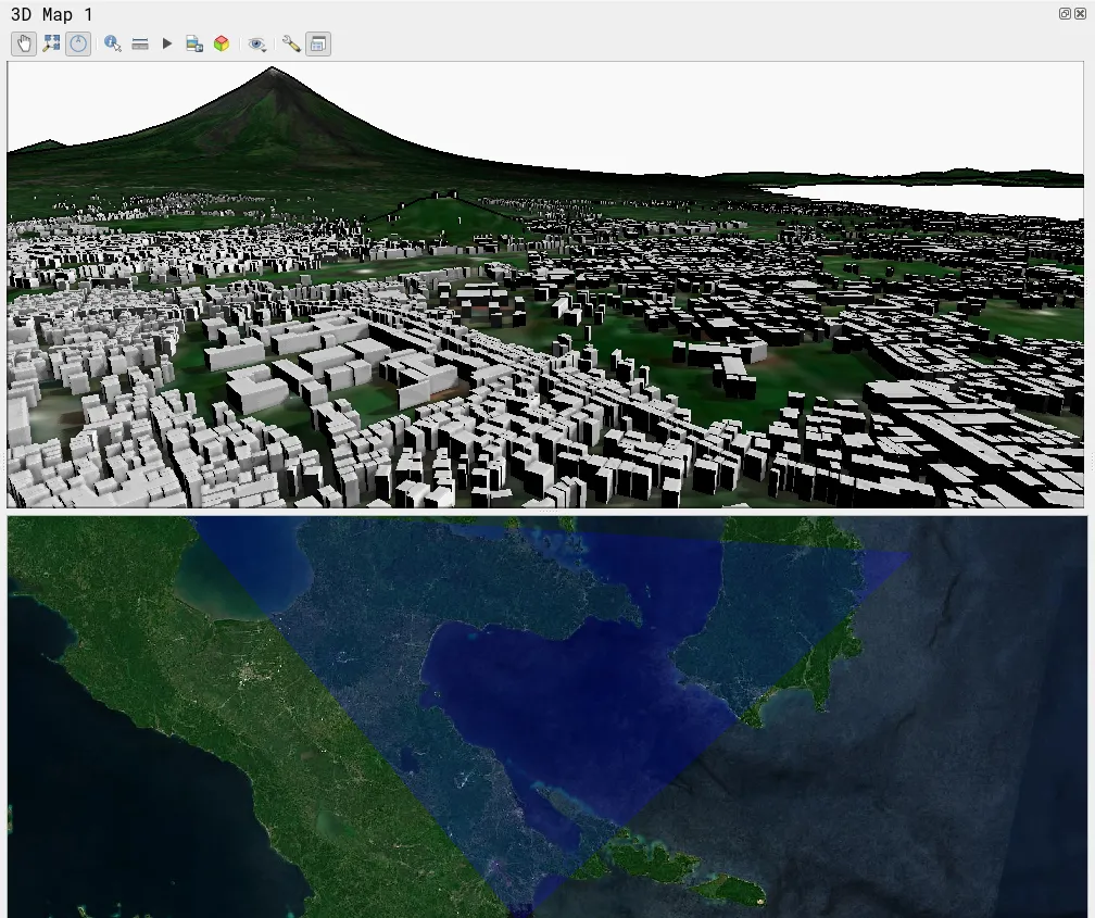
The native 3D support in QGIS allows you to render rasters, vectors, and mesh layers. It also provides you with methods for visualizing data in 3D depending on data type. For example, you can render points, extrude polygons, use DEMs as terrain, and even load external 3D models.

To access and manage 3D views in QGIS, go to View > 3D Map Views.

PRO-TIP

To learn more about 3D Map Views in QGIS, you may refer to: https://docs.qgis.org/latest/en/docs/user_manual/map_views/3d_map_view.html

In this exercise, we will visualize the the province of Albay in 3D using a DEM and extrude buildings from OpenStreetMap.

1. Load the osm_buildings, albay_srtm_32651, and satellite imagery of your choice.

Figure 4.1.1.1. osm_buildings, albay_srtm_32651, and satellite imagery layers loaded in QGIS

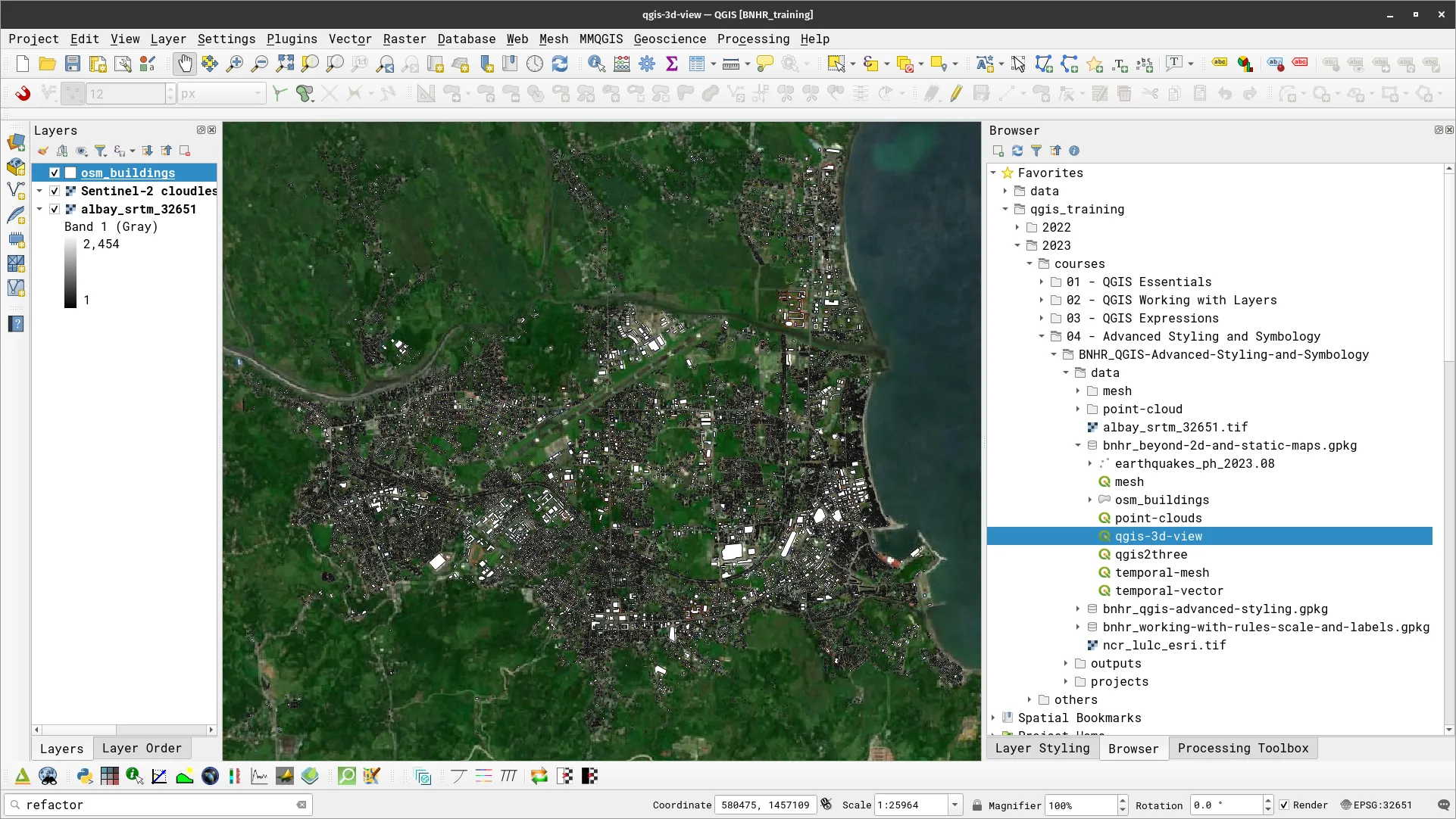
Opening a new 3D map view

2. Open a new 3D Map View in View > 3D Map Views > New 3D Map View. Add this map view to the QGIS interface.
3. You can edit or rename this new Map View in the same menu.
4. Notice that the 3D Map View is a bit bare. Next, you will edit its configuration to add the 3D information.
5. To configure the 3D view, click on the configure (wrench) button in the map view toolbar.

Figure 4.1.1.2. 3D map view toolbar

Figure 4.1.1.3. New 3D map view added to QGIS

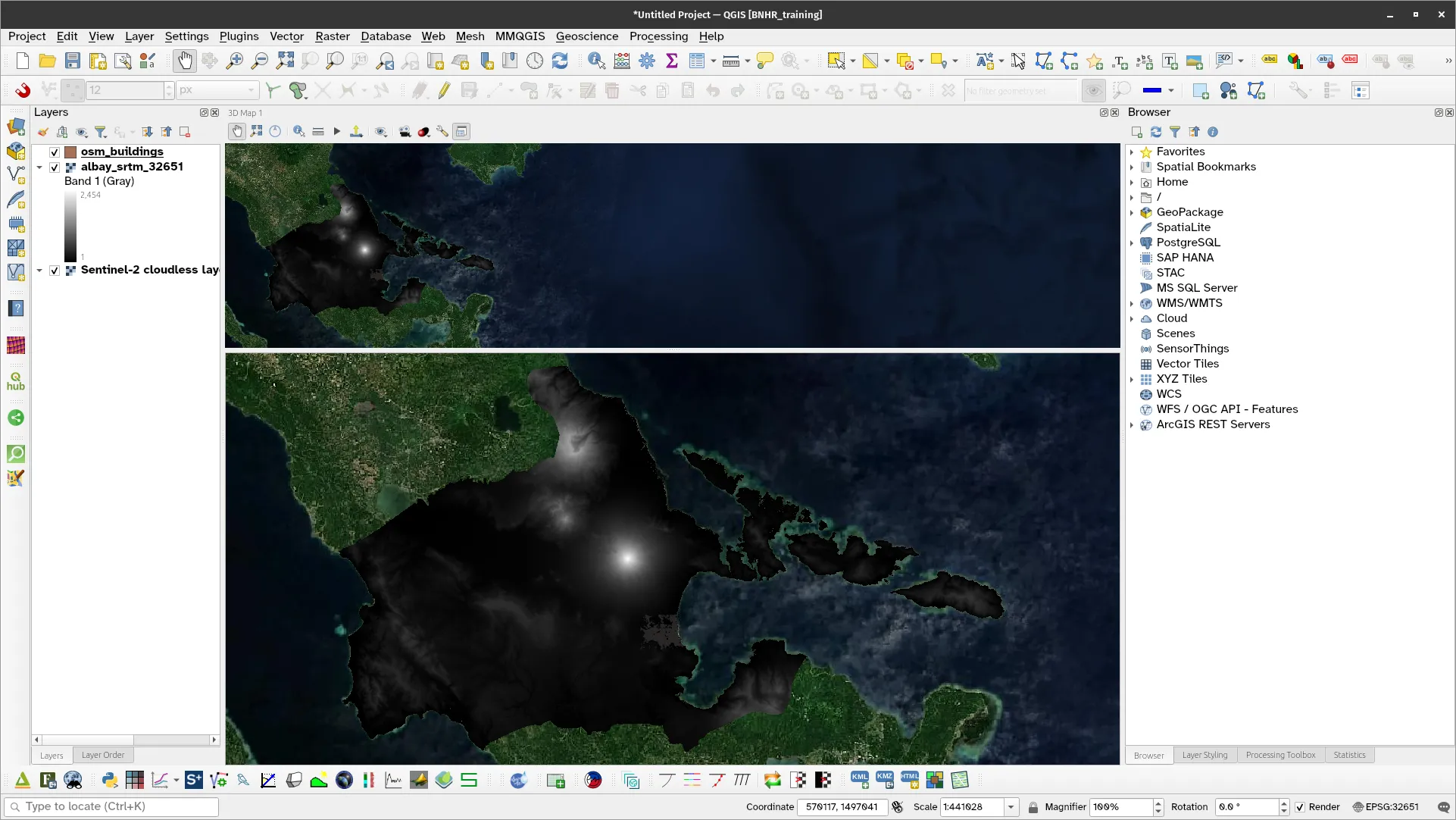
Use a DEM as the terrain

6. Instead of having a flat surface in your 3D view, you can specify a DEM to serve as the terrain. In this case, use the following parameters for Terrain:
   1. Type: DEM (Raster)
   2. Elevation: albay_srtm_326451

Figure 4.1.1.4. Terrain parameters

NOTE

Make sure that the Coordinate Reference System (CRS) that your data/project is using is a projected CRS (i.e. units are linear, in meters, km, etc.)

Apply 3D styles to a vector layer

7. Next, you can also apply different styles for your vector layers in 3D. For example, we can add an extrusion to the osm_buildings layer. In this case, we will give all buildings the same extrusion value (20).

NOTE

If you have data about building heights, you can use it as the data-defined value for extrusion.

8. Go to the 3D View tab of the Symbology or Layer Styling panel of the osm_buildings layer and add the following parameters:

Figure 4.1.1.5. Parameters for 3D view of the osm_buildings layer

PRO-TIP

To learn more about the other parameters, refer to: https://docs.qgis.org/latest/en/docs/user_manual/map_views/3d_map_view.html

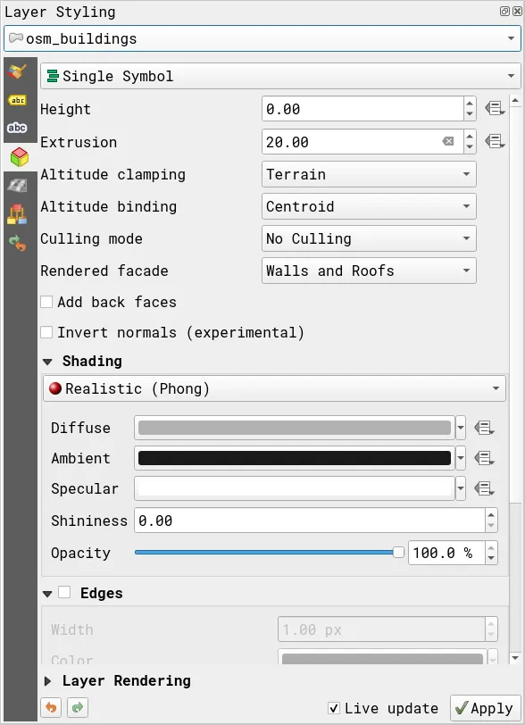
9. Your 3D view should look similar to the one below.

Figure 4.1.1.6. 3D view using albay_srtm_32651 DEM as the terrain and with osm_buildings extruded

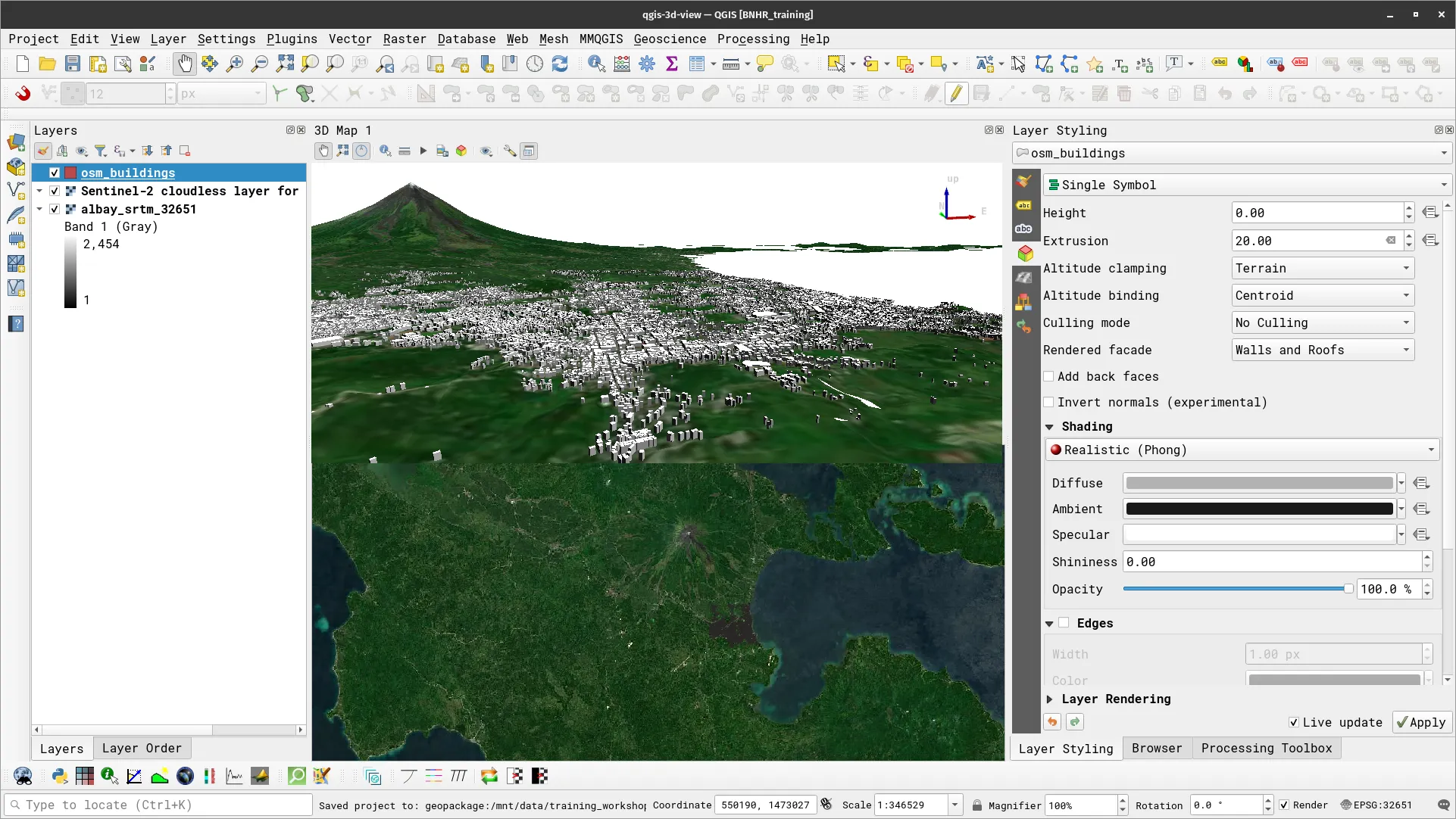
10. Try to move around and navigate the 3D scenes.

Shadows, Eye Dome Lighting, and Ambient Occlusion

QGIS 3D views also have built in support for shadows, eye dome lighting, and ambient occlusion that can improve your 3D visualizations.

11. To add these effects, go to the Configure tool and check the effect you want to activate.

Figure 4.1.1.7. 3D view with shadows, eye dome lighting, and ambient occlusion

NOTE

You can add the 3D view in your Print Layouts.

Exercise 4.1.2. Qgis2threejs plugin

PRO-TIP

For our training participants, you can load the completed/styled layer by loading the qgis2threejs project found inside bnhr_beyond-2d-and-static-maps.gpkg

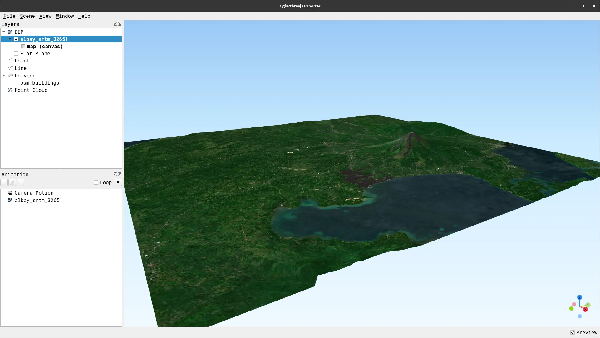
The three.js library is a popular, open source, JavaScript 3D library. Aside from general 3D work, you can use three.js to create 3D web maps. You can do this by writing code yourself or you can leverage QGIS to create your 3D maps with three.js using the Qgis2threejs plugin.

https://plugins.qgis.org/plugins/Qgis2threejs/

NOTE

If you notice some incompatibility between the native 3D view and theQgis2threejs plugin. For example, if you want to use the plugin to preview your 3D map and it doesn’t work, try to remove all the 3D views/canvases and restart QGIS.

In this exercise, you will visualize the same data in the previous exercise but using the Qgis2threejs plugin.

1. Load the osm_buildings, albay_srtm_32651, and satellite imagery of your choice.
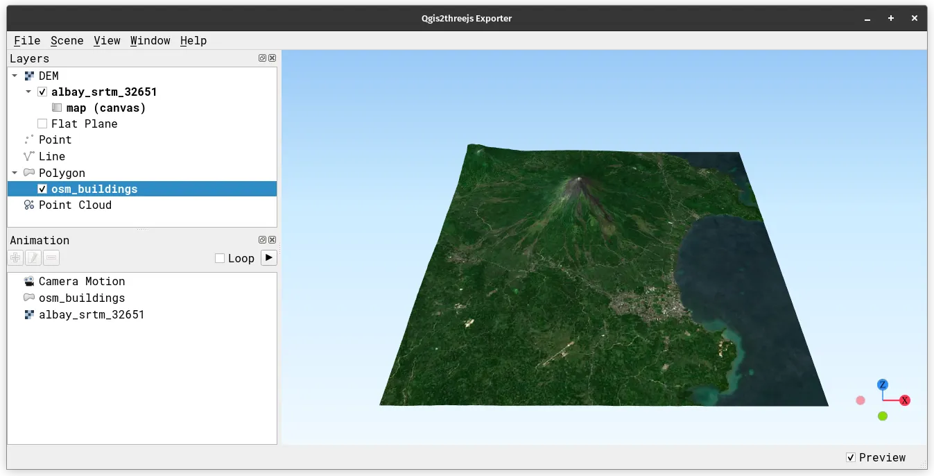
2. Run the Qgis2threejs plugin in Web > Qgis2threejs > Qgis2threejs Exporter

Figure 4.1.2.1. The Qgis2threejs windown

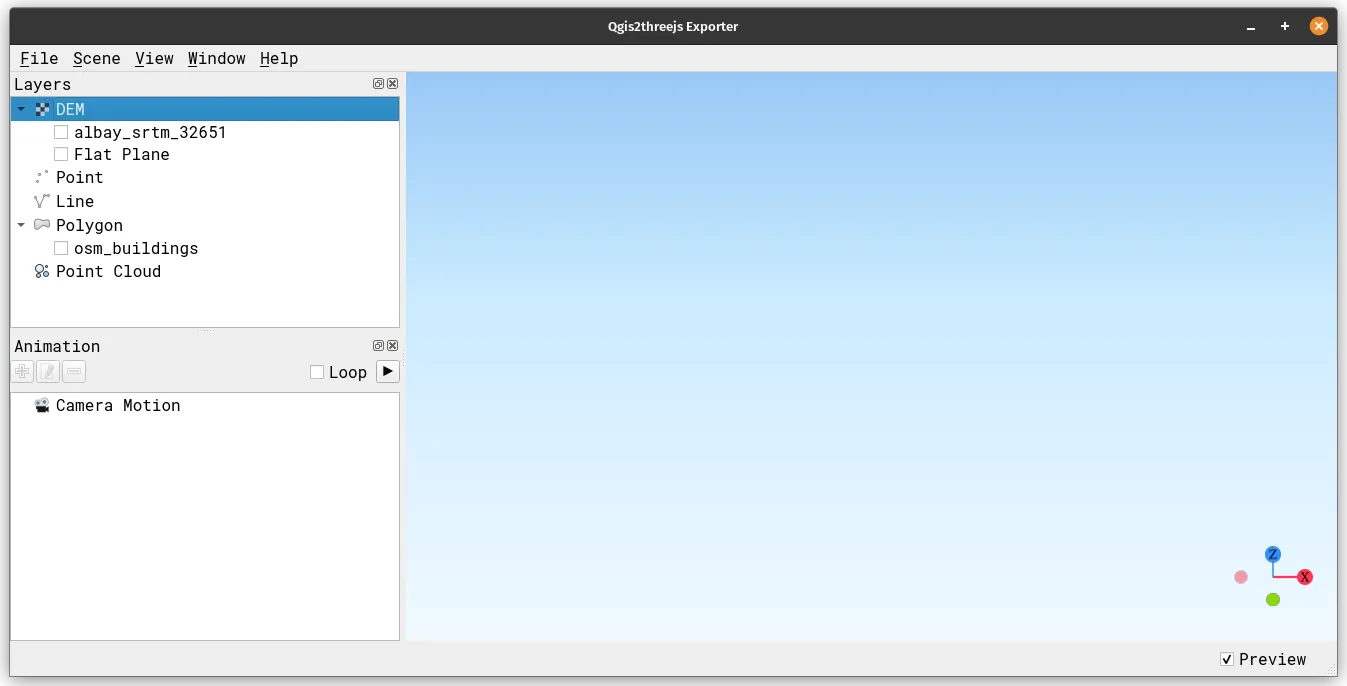
3. Check the albay_srtm_32651 and osm_buildings. What happened?

Figure 4.1.2.2. Preview of albay_srtm_32651 and osm_buildings

NOTE

Notice that Qgis2threejs renders the extent shown in the Map canvas.

Editing layer parameters

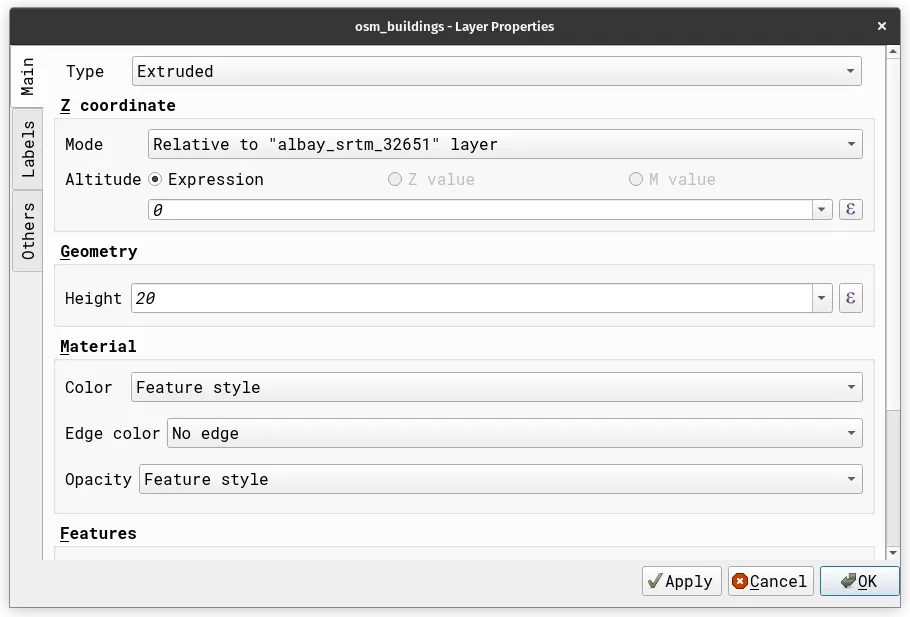
1. You can edit layer parameters by Right-clicking on the layer > Properties… Edit the properties of osm_buildings so that it is extruded (has a height above the ground) by 20m. Use the parameters below.

Figure 4.1.2.3. osm_buildings properties

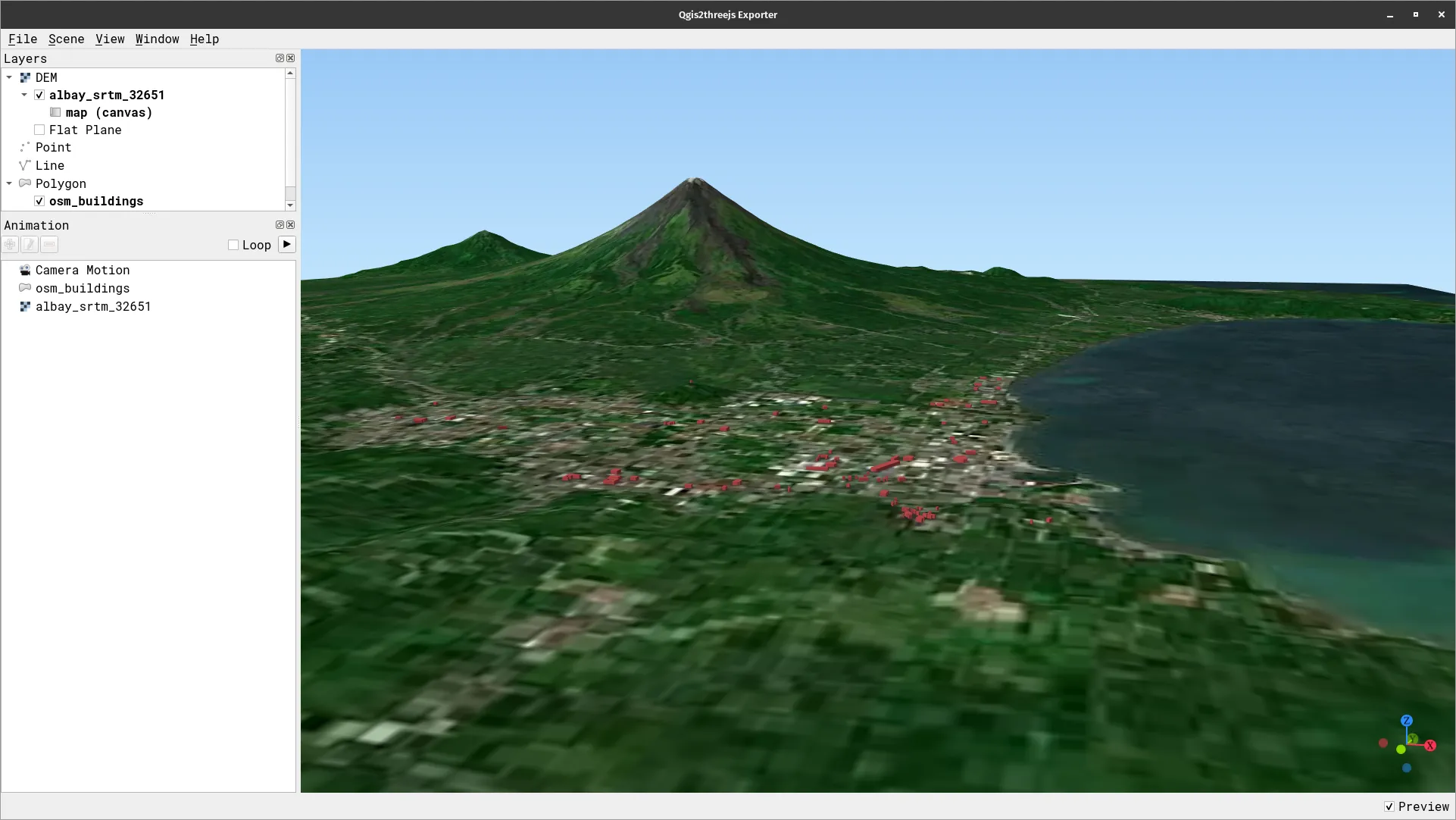
2. Zoom into the osm_buildings layer. Your preview should look similar to the one below.

Figure 4.1.2.4. 3D preview using Qgis2threejs plugin

TRY IT YOURSELF

You can use the qgis2threejs plugin to export your 3D scene as a 3D web map. This 3D web map can easily be opened in any browser or stored in any web server to make it accessible online.

Point clouds

QGIS has both native support for visualizing and processing point clouds.

A point cloud is a three-dimensional representation of a space, comprised of numerous individual data points (as suggested by its name). Point clouds commonly include millions if not billions of points. Examples of point clouds are datasets obtained from drone/UAV surveys and photogrammetry.

Each point within the cloud possesses x, y, and z coordinates as well as additional attributes derived from the capture process, such as color values or intensity. These attributes enable functionalities like displaying point clouds in various colors. In QGIS, point clouds can be harnessed to create three-dimensional depictions of landscapes or other spatial environments.

QGIS offers support for two data formats: Entwine Point Tile (EPT) and LAS/LAZ. When dealing with point clouds, QGIS consistently saves data using the EPT format. EPT, a storage format, involves multiple files stored within a shared directory. EPT incorporates indexing for swift data access. For comprehensive insights into the EPT format, refer to the entwine homepage.

If the data exists in LAS or LAZ format, QGIS undertakes a conversion to EPT during the initial load. Depending on file size, this conversion process may consume some time. During this conversion, a subfolder adhering to the scheme “ept_ + name_LAS/LAZ_file” is generated within the folder containing the LAS/LAZ file. Should such a subfolder already exist, QGIS promptly loads the EPT, resulting in reduced loading times.

Exercise 4.2. Visualizing point clouds in QGIS

PRO-TIP

For our training participants, you can load the completed/styled layer by loading the point-clouds project found inside bnhr_beyond-2d-and-static-maps.gpkg or or you can watch this exercise at: https://www.youtube.com/watch?v=nGXA1BhCh_Q

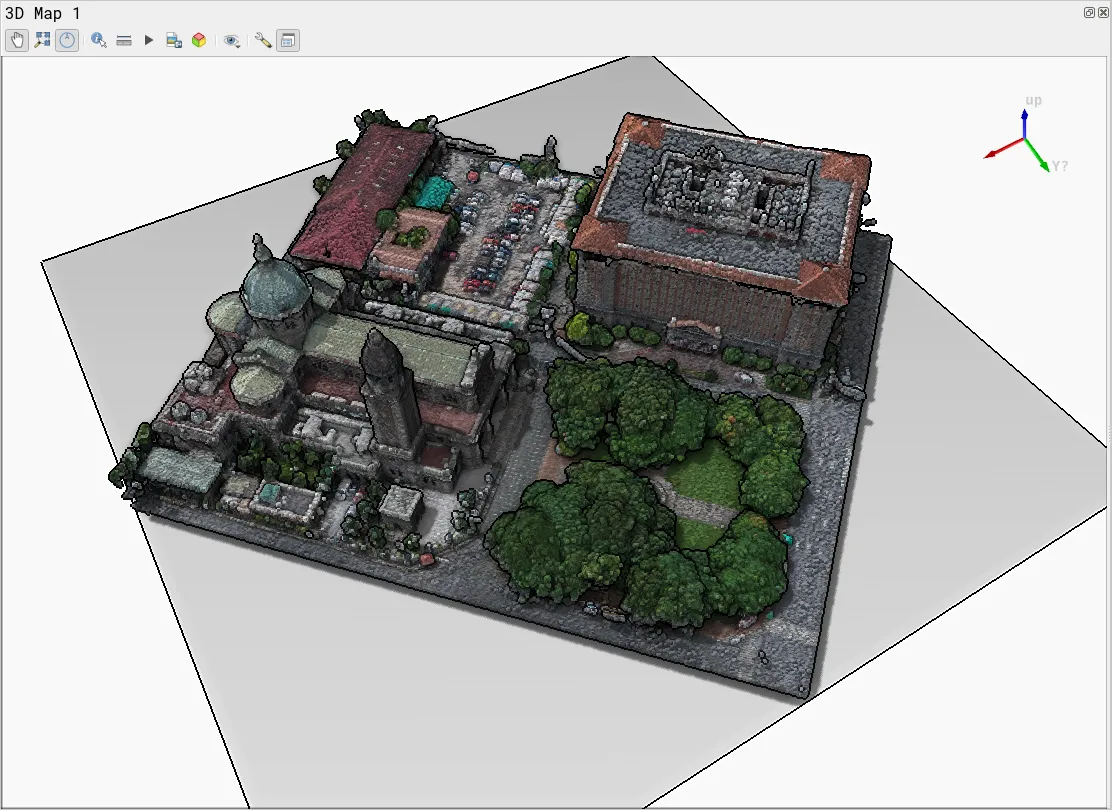
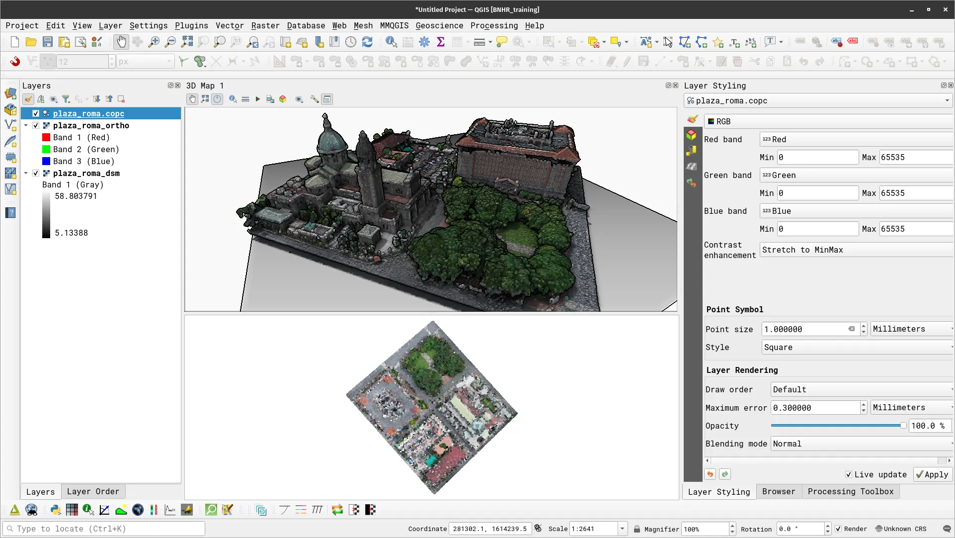
In this exercise, you will load a point cloud of Plaza Roma, Philippines in QGIS and apply some basic styling.

1. Load the the plaza_roma.copc layer.

Figure 4.2.1. plaza_roma point cloud loaded in QGIS

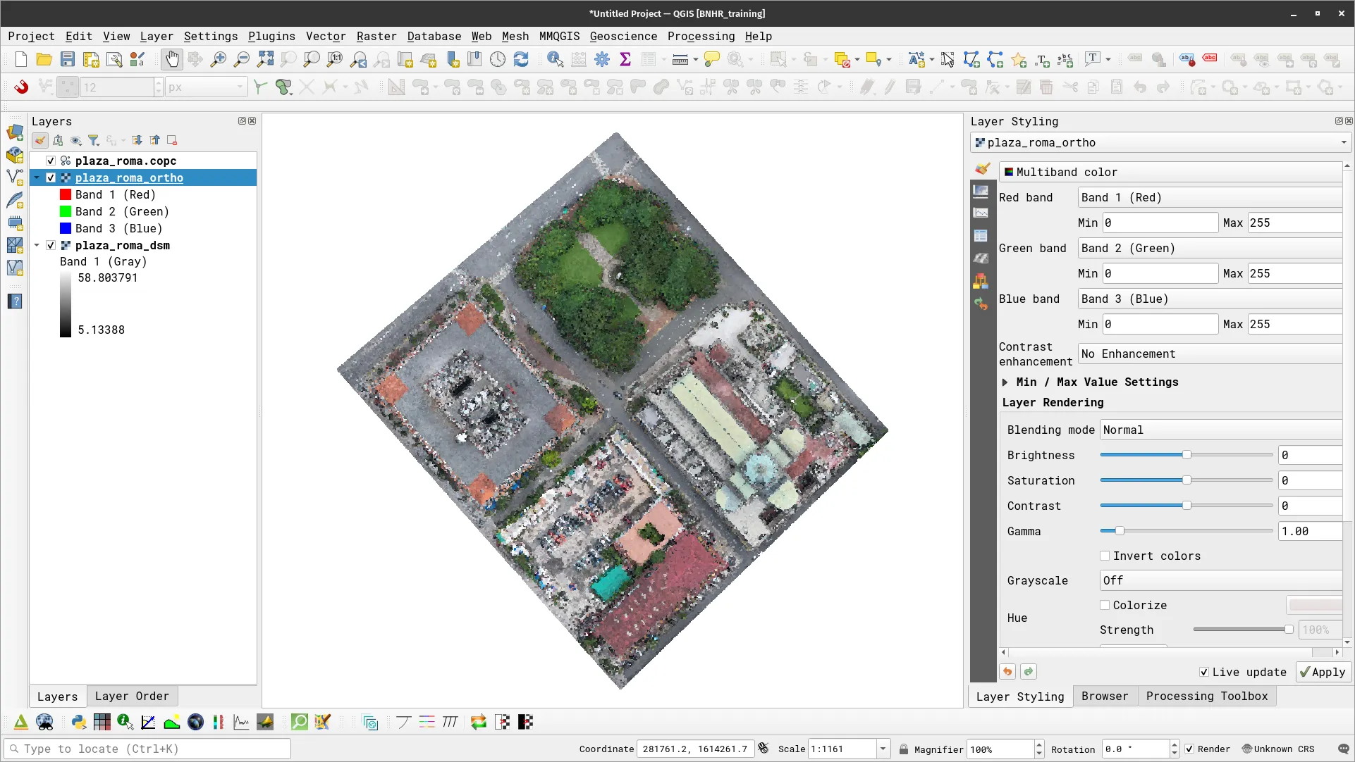
2. Create a new 3D map view.

Figure 4.2.2. Plaza Roma point cloud viewed in 3D

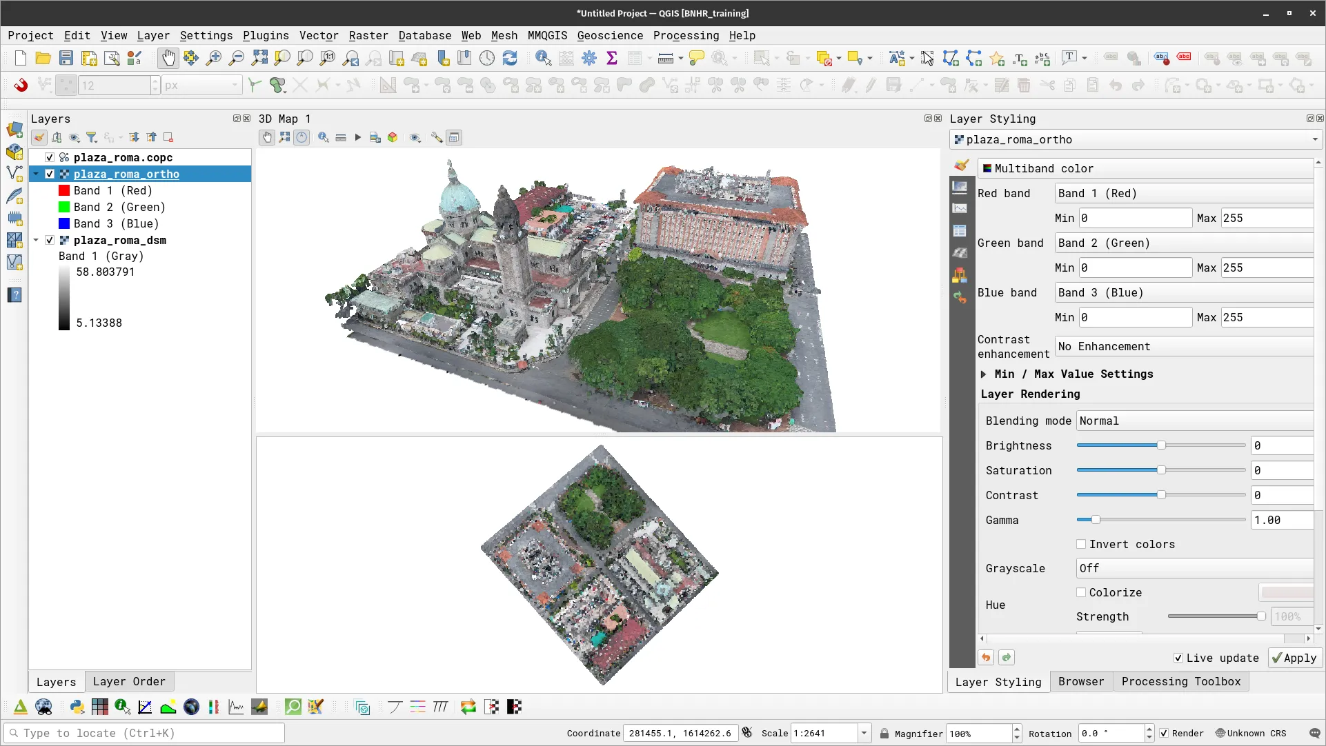
3. Apply some basic effects.

Figure 4.2.3. Plaza Roma point cloud with shadows, EDL, and ambient occlusion

TRY IT YOURSELF

Use other effects and point cloud data.

Mesh data

QGIS also has native support for mesh data.

A mesh is an unstructured grid with spatial and often temporal components. The spatial part comprises vertices, edges, and faces, forming shapes in 2D or 3D space:

• Vertices: Represent XY(Z) points, following the layer’s coordinate reference system.
• Edges: Connect pairs of vertices.
• Faces: Consist of sets of edges forming closed shapes, typically triangles, quadrilaterals (quads), and occasionally polygons with more vertices.

Mesh layers can have varying structures based on these components:

1. 1D Meshes: Composed of vertices and edges. Edges can carry data (scalars or vectors). Useful for modeling urban drainage systems.
2. 2D Meshes: Comprise faces with triangles or unstructured quads.
3. 3D Layered Meshes: Stacked 2D meshes extruded vertically (levels) with the same topology. Can change over time. Data is typically defined in volume centers or parametric functions.

QGIS employs the Mesh Data Abstraction Library (MDAL, https://www.mdal.xyz/) drivers to access mesh data and inherently supports multiple formats. MDAL provides a single data model for supported mesh data similar to what GDAL does for rasters and vectors. The available functions that you can do with mesh layers depends on the format and structure.

PRO-TIP

To learn more about working with Mesh Data in QGIS, you can refer to: https://docs.qgis.org/latest/en/docs/user_manual/working_with_mesh/mesh_properties.html

Exercise 4.3. Loading and visualizing mesh data

PRO-TIP

For our training participants, you can load the completed/styled layer by loading the mesh project found inside bnhr_beyond-2d-and-static-maps.gpkg.

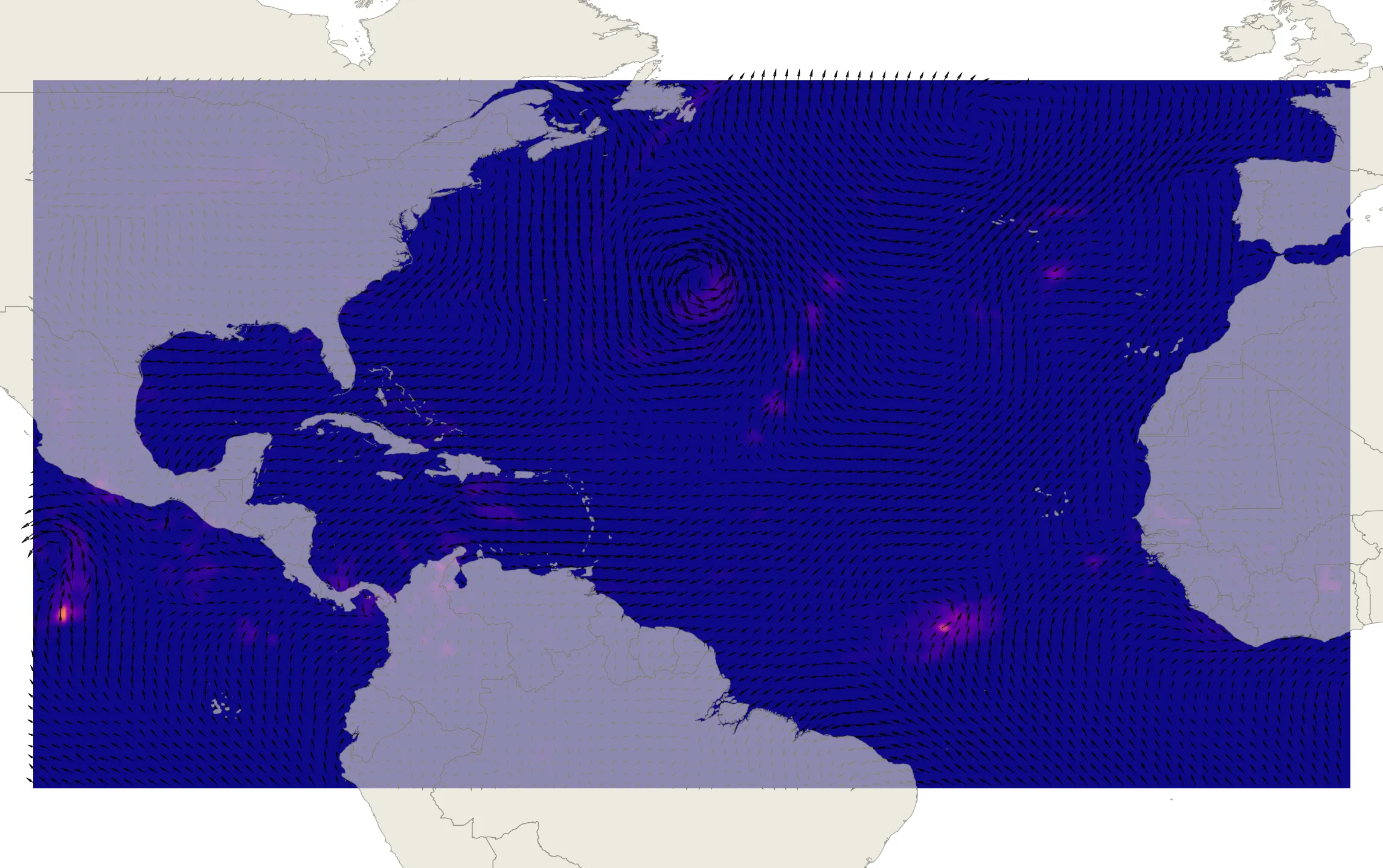
In this exercise, you will load a mesh dataset of hurricane Michael in QGIS and apply some basic visualizations.

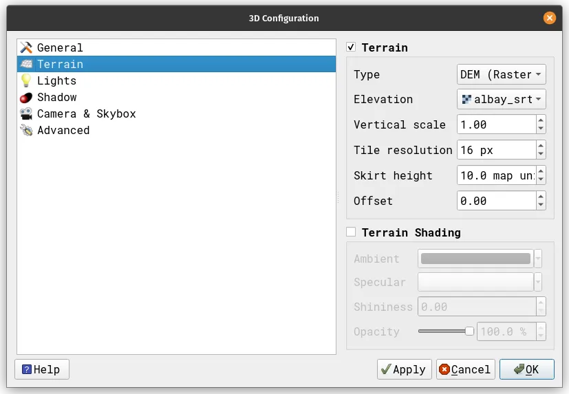
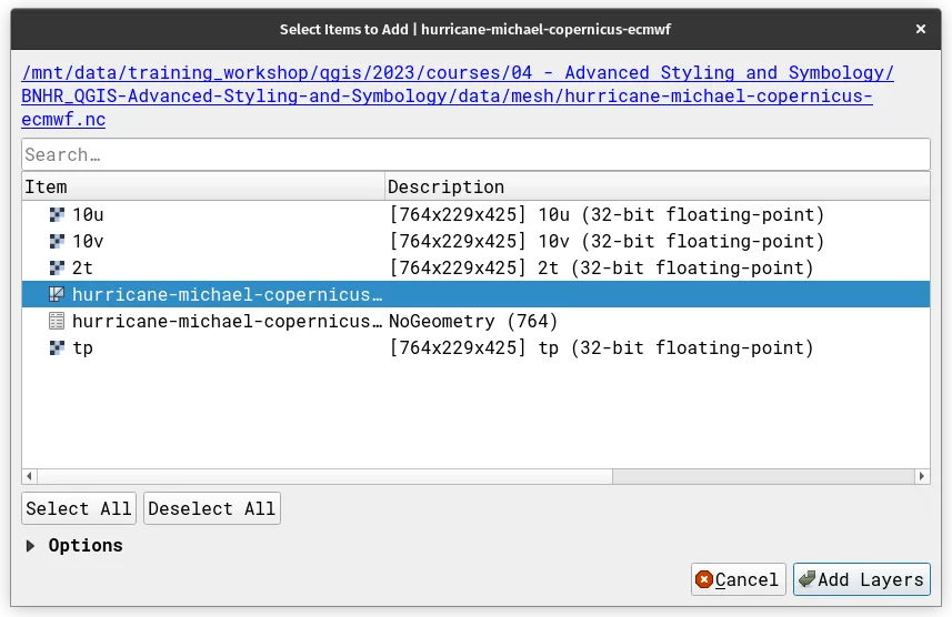
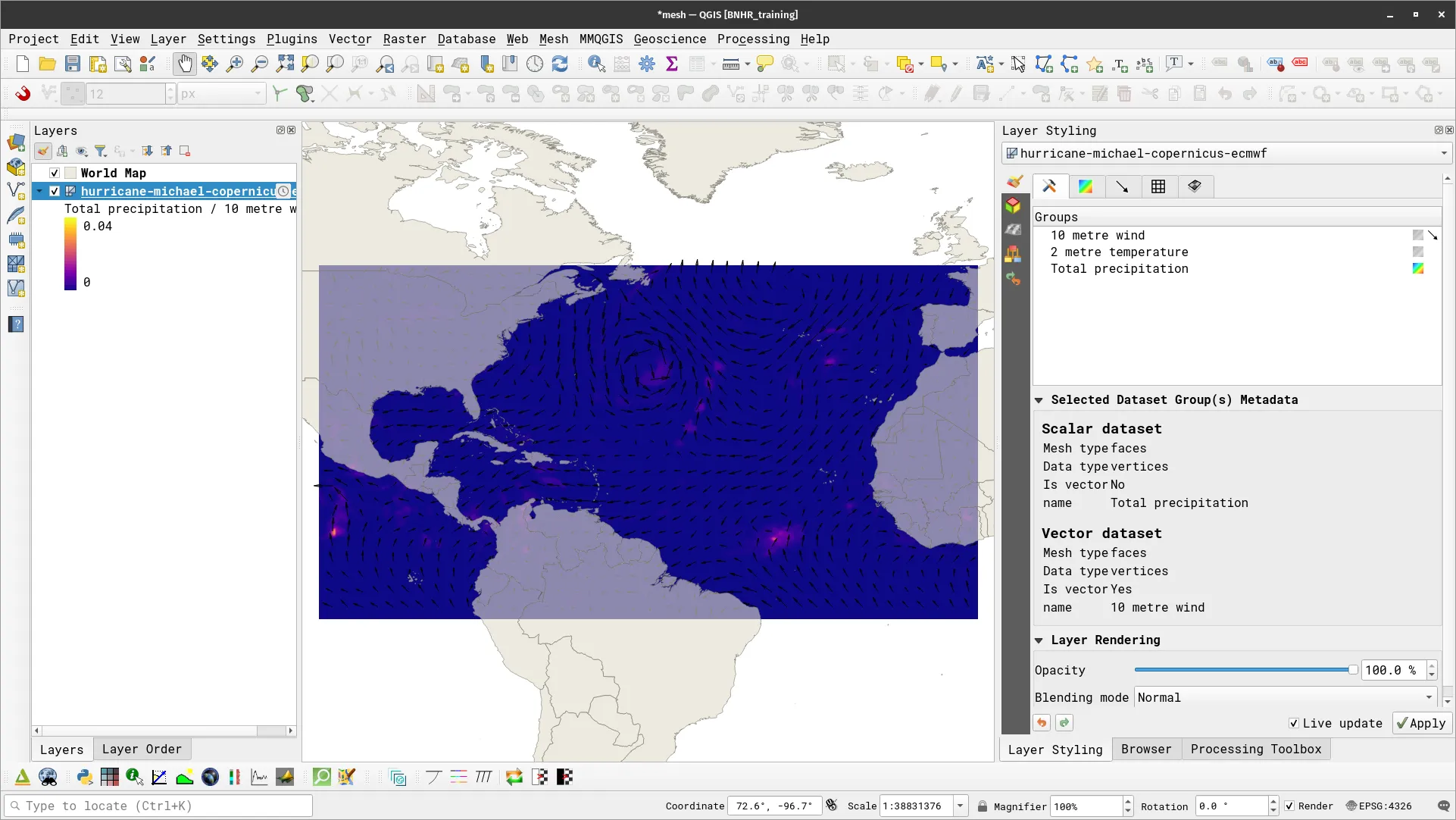
1. Load the hurricane-michael-copernicus-ecmwf.nc file in QGIS. Select the mesh data (shown below).

Figure 4.3.1. Loading the mesh data in QGIS

2. The layer you loaded should look similar to the one below.

Figure 4.3.2. Hurricane Michael mesh data loaded in QGIS

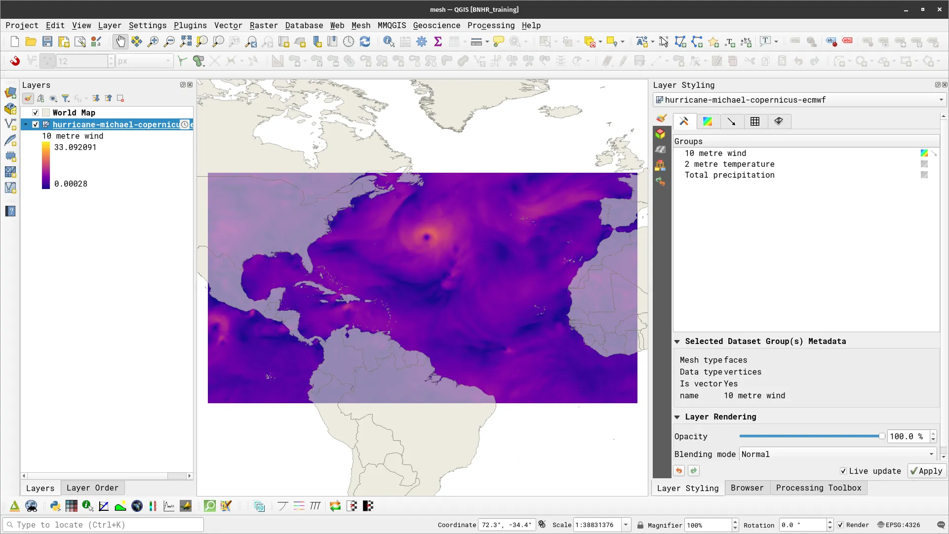
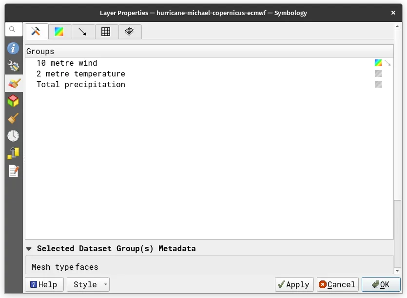
3. Notice that the layer has several groups that you can style (10 metre wind, 2 metre temperature, Total precipitation). These are information stored in the mesh data that we can show individually. Notice also that the 10 metre wind group has 2 icons to the right of it. The first pertains to Contours and the second pertains to Vectors. We can visualize and enable these to separately as well.

Figure 4.3.3. Styling parameters for the Hurricane Michael mesh data

4. Do the following:
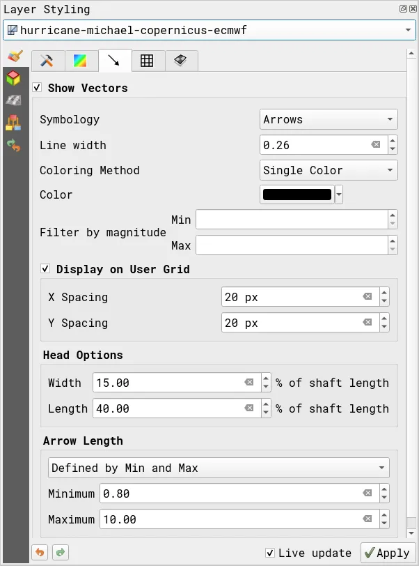
   1. Enable Total Precipitation contour and the 10 metre wind vector. Go to the vector tab and apply the following parameters:
      1. Check Display on User Grid
         • X Spacing: 20 px
         • Y Spacing: 20 px

Figure 4.3.4. Vector styling parameters

5. Your map canvas should show both the total precipitation (as contours) and 10-meter wind (as vectors) like below.

Figure 4.3.5. Visualization showing the total precipitation and 10 meter wind vectors

TRY IT YOURSELF

Try to play around with other parameters for visualizing the mesh dataset.

SOMETHING TO THINK ABOUT

Notice that the hurricane-michael-copernicus-ecmwf layer has a clock icon next to it on the Layers panel. What could this mean?

Temporal visualization

QGIS 3.14 introduced the Temporal Controller that provides native support for viewing temporal data in QGIS. Prior to this, the Time Manager plugin provided a similar functionality.

Using the Temporal Controller, you will be able to view and export “snapshopts” of data along specific time intervals. You can also combine them to create animations.

The Temporal Controller supports temporal information stored in different file formats such as rasters, meshes, and vectors.

To enable Temporal support, open a layer’s Properties and go to the Temporal tab. Depending on the kind of data it is, you will see different options for configuring temporal support. If successfully configured, you should see this icon () next to the layer.

Mesh data

Exercise 4.4.1. Temporal visualization of mesh data

PRO-TIP

For our training participants, you can load the completed/styled layer by loading the temporal-mesh project found inside bnhr_beyond-2d-and-static-maps.gpkg.

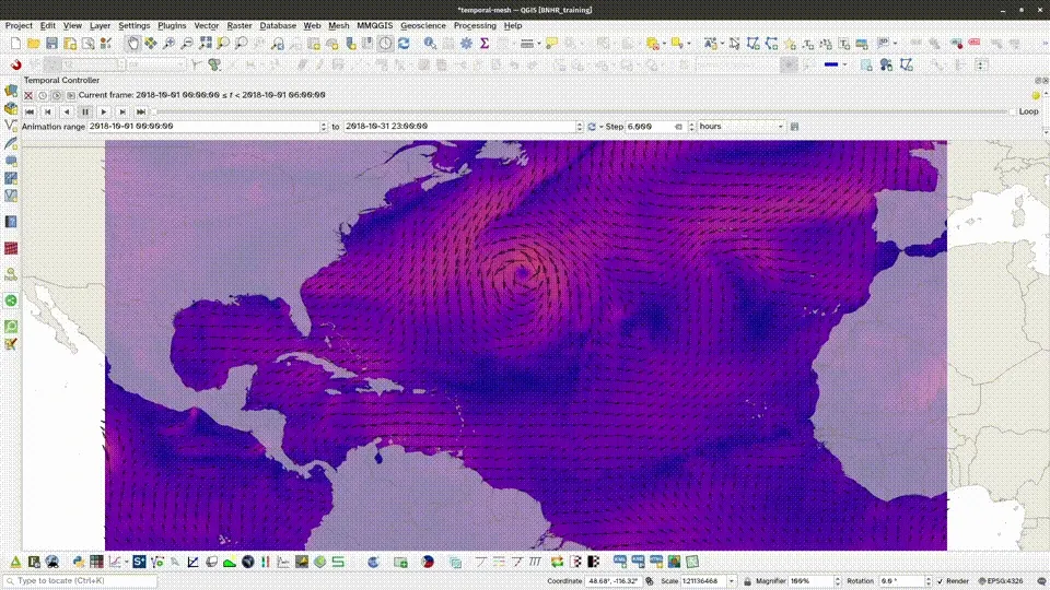
The mesh data we loaded in the previous exercise actually contains information for about the hurricane at different times—e.g. hourly data from October 1-31, 2018. We can use this information to view the status of the hurricane over time.

Figure 4.4.1.1. Hurricane michael mesh data with the “temporal” icon

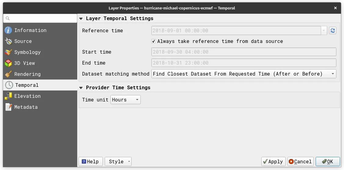
1. Edit the temporal configuration of the layer by opening its Properties > Temporal tab and apply the following settings.

Figure 4.4.1.2. Temporal settings for hurricane michael mesh data

2. Next, we open the Temporal Controller Panel by clicking on the clock button () in the Map Navigation Toolbar.

Figure 4.4.1.2. Temporal settings for hurricane michael mesh data

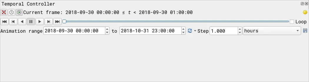
3. The Temporal Controller Panel has several functions that allow you to configure temporal navigation. To enable temporal navigation, click on the right-most button (with play button).
4. Make sure that the Animation range values are correct—i.e. they correspond to the dates available in your data.
5. The Step parameter defines how long each step/snapshot will be.

Figure 4.4.1.4. Temporal Controller Panel

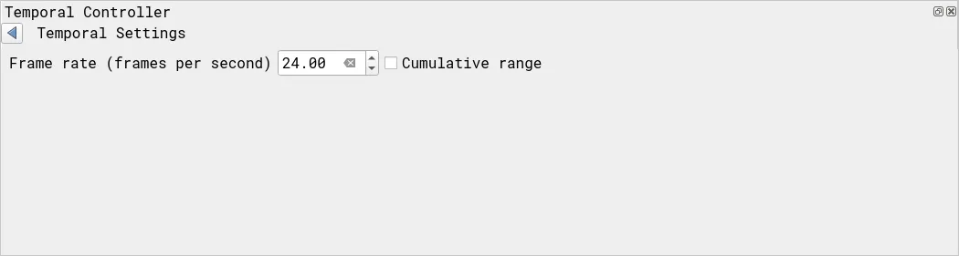
6. If your animation is slow, you can also edit the framerate by clicking on the gear button on the upper right of the Temporal Controller Panel.

Figure 4.4.1.5. Frame rate increased to 24 per second

7. With your animation properly configured, try to see how it looks like by playing the animation.

Figure 4.4.1.6. Animated temporal view of hurricane michael mesh data

8. Feel free to modify the parameters to suit your needs.
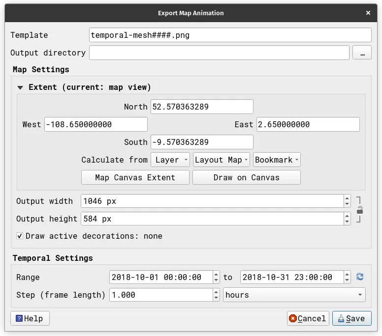
9. You can also save the frames of the animation as a set of images that you can then use to create videos, GIFs, and other animations. To do this, click on the Save button in the Temporal Controller panel (next to the Step parameter).

Figure 4.4.1.7. Saving the animation frames as images

Vector data

Exercise 4.4.2. Temporal visualization of vector data (mapping earthquakes)

PRO-TIP

For our training participants, you can load the completed/styled layer by loading the temporal-vector project found inside bnhr_beyond-2d-and-static-maps.gpkg.

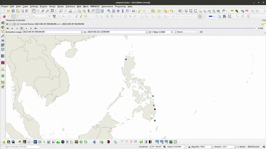
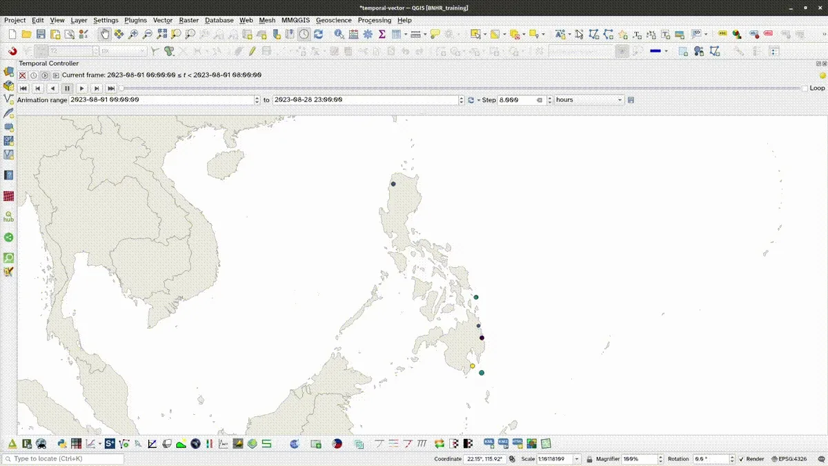
You can also use the temporal controller for styling vectors. This is especially useful if you want to see not just where but when events occur. In this exercise, you will visualize earthquakes in the Philippines for the month of August 2023 from data gathered by PHIVOLCS.

1. Load the earthquakes_ph_2023.08 data in QGIS.

Figure 4.4.2.1. Earthquakes in the Philippines (August 2023)

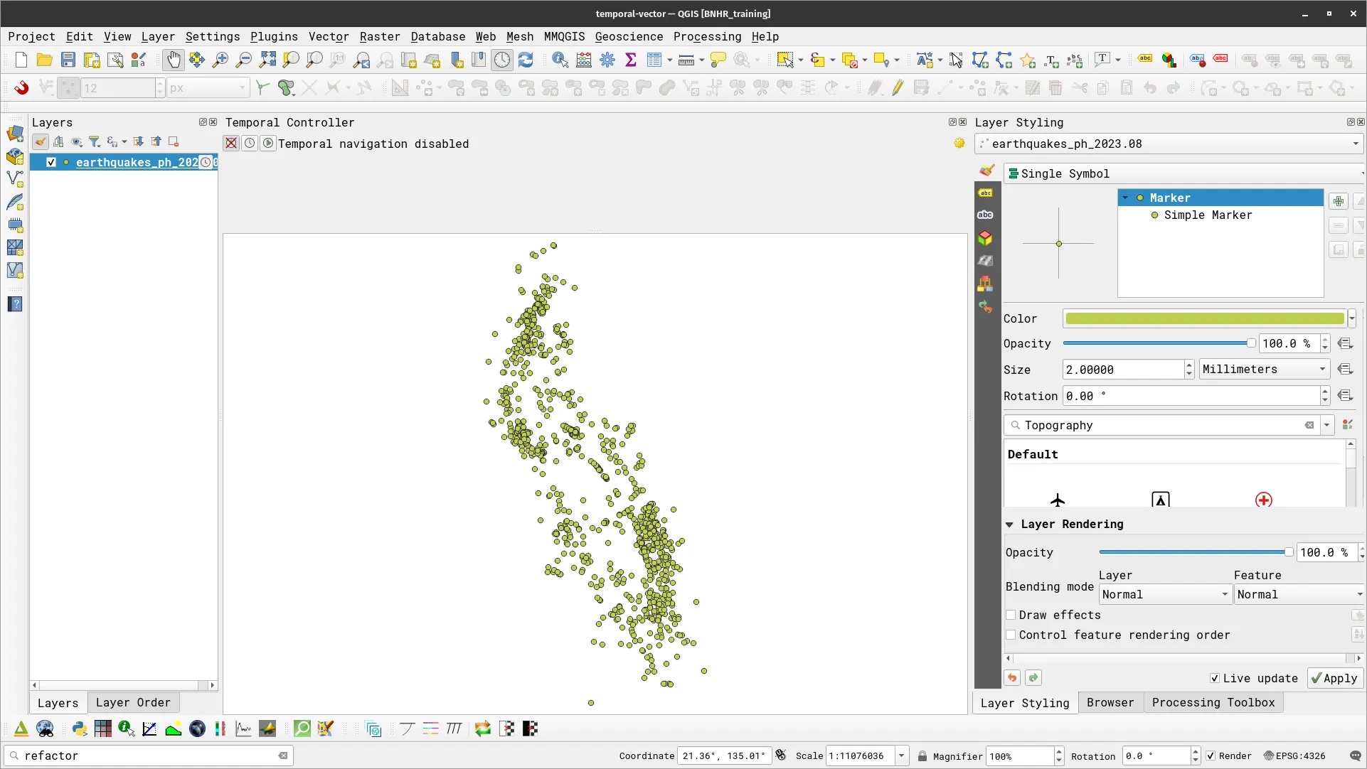
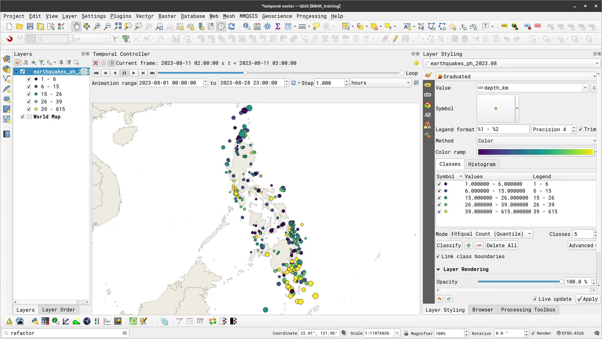
2. Check the attribute table/fields of this layer. Notice that it has fields for magnitude (mag), earthquake depth (depth_km), and the date + time of the earthquake (datetime).

Figure 4.4.2.2. Fields of the earthquake data

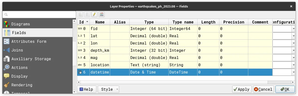
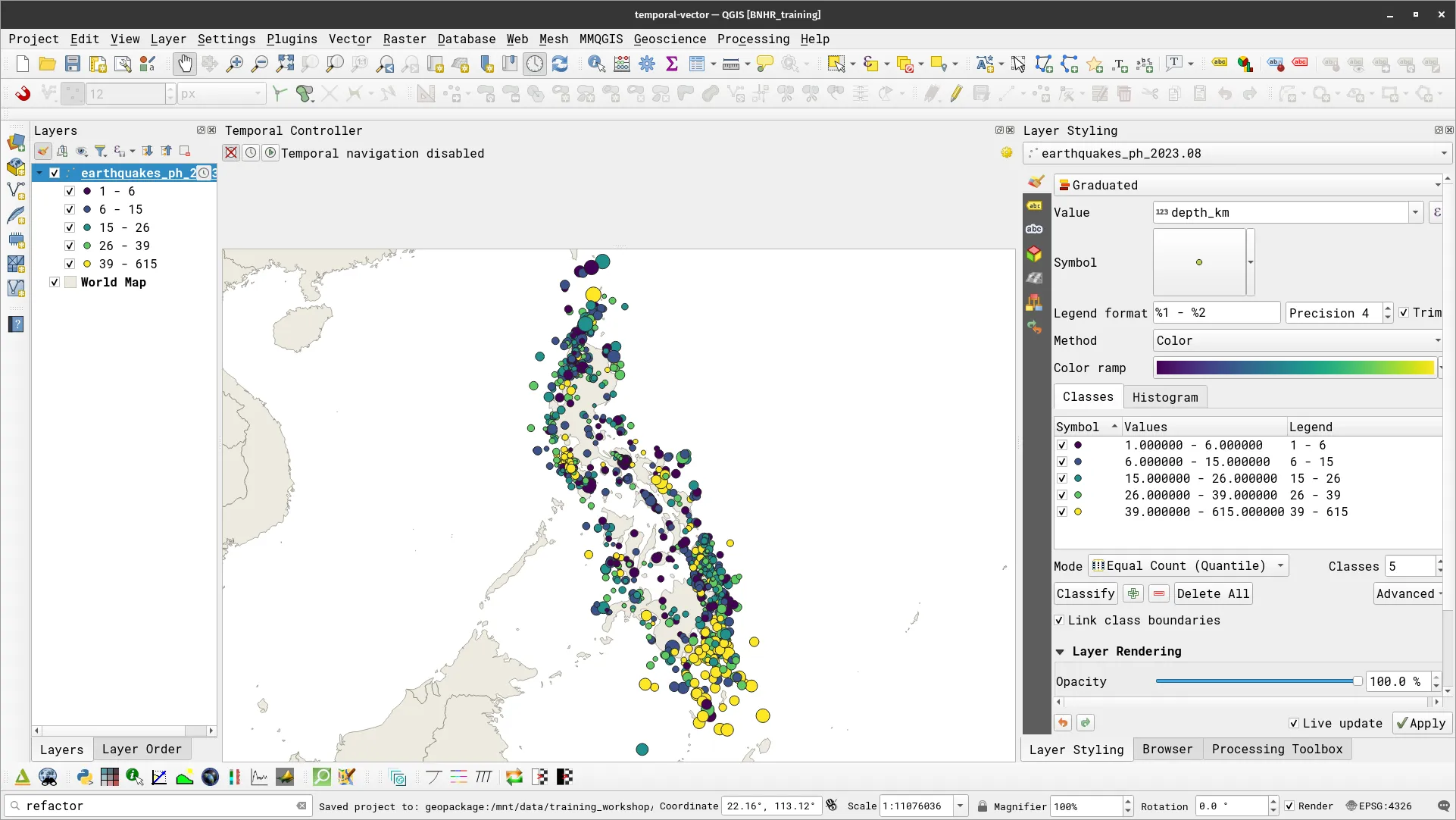
3. Style the layer such that the size indicates the magnitude (mag) and the color indicates the depth (depth_km). You can utilize a Graduated symbology with data-defined size.

Figure 4.4.2.3. Earthquakes in the Philippines (August 2023) styled

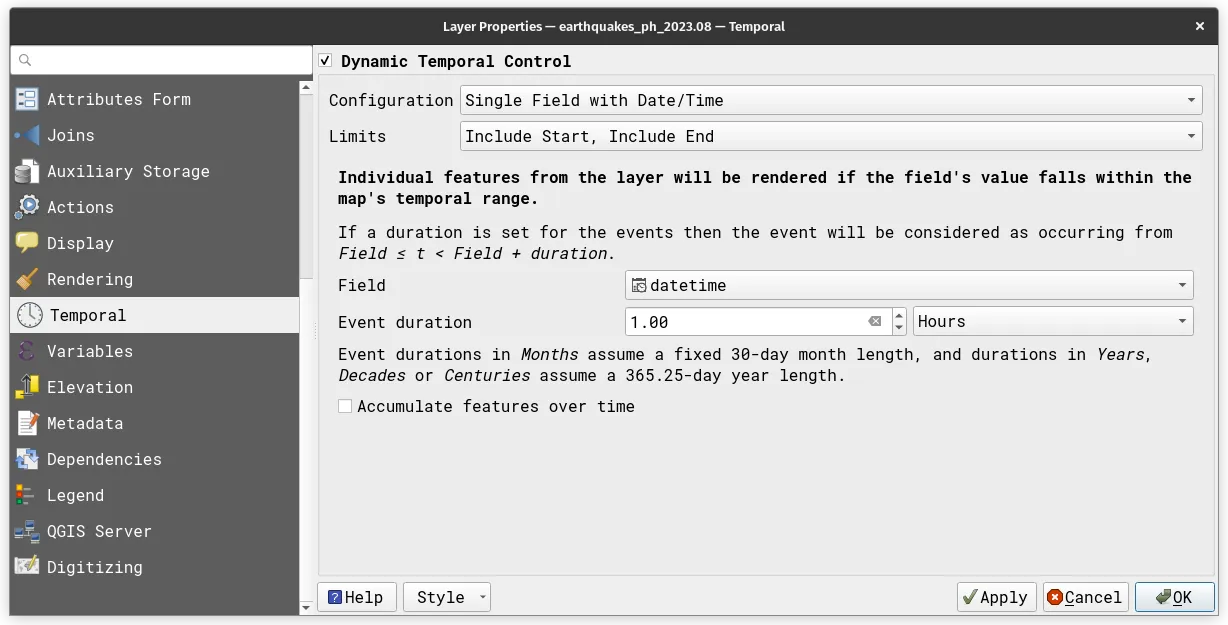
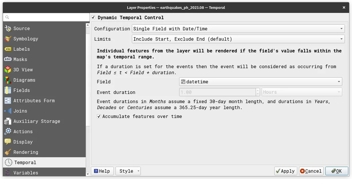
4. Open the Temporal tab in the layer’s Properties and check Dynamic Temporal Control. Edit the Configuration as Single Field with Date/Time, Limits as Include Start, Include End, Field is datetime, and Event duration is 1.00 Hours.

Figure 4.4.2.4. Temporal parameters for the earthquake layer

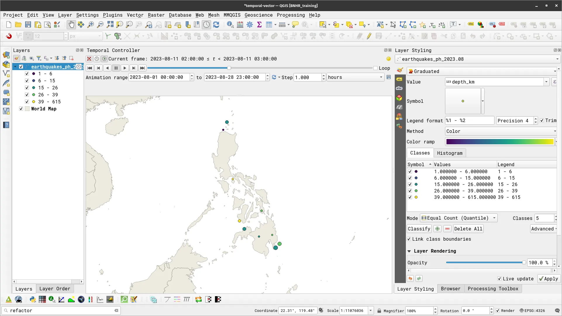
5. Open the Temporal Controller Panel. Make sure that the Animation range is correct (e.g. between 2023-08-01 and 2023-08-28). For now, use 1.00 hours as the step but you can change it later. Play the temporal animation, what do you notice?

Figure 4.4.2.5.a. The Temporal Controller showing a “snapshot” of the data for the specific time

Figure 4.4.2.5.b. The Temporal Controller showing a “snapshot” of the data for the specific time

PRO-TIP

The temporal controller can show a “snapshot” in time of the data but it can also show the “cumulative” data up to that time.

6. What if you want to show the cumulative earthquakes over the course of the month? To do this, open the Temporal tab again and check Accumulate Feature over time

Figure 4.4.2.6. Enabling feature accumulation in the temporal controller

7. Run the temporal animation again. Run the temporal animation again. What changed?

Figure 4.4.2.7.a. The Temporal Controller showing a accumulation of the data (earthquakes) over time

Figure 4.4.2.7.b. The Temporal Controller showing a accumulation of the data (earthquakes) over time

Certification and support

LOOKING FOR CERTIFICATION AND SUPPORT?

We offer additional resources, certificates, official QGIS certification, ongoing support, and other perks to those who avail of our paid courses.

Contact us or sign-up to our courses if you are interested in having this as an instructor-led or self-paced course.